Summary
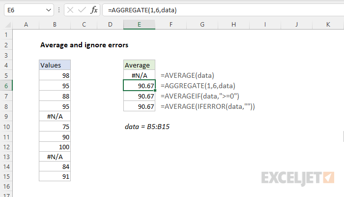
To average values in a range while ignoring any errors that may exist, you can use the AVERAGEIF or AGGREGATE function, as described below. In the example shown, the formula in E6 is:
=AGGREGATE(1,6,data)
where data is the named range B5:B15.
Generic formula
=AGGREGATE(1,6,data)
Explanation
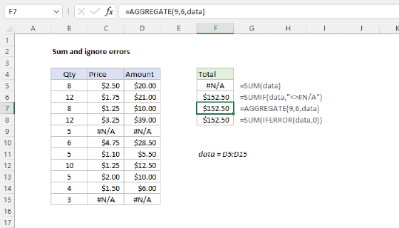
In this example, the goal is to average a list of values that may contain errors. The values to average are in the named range data (B5:B15). Normally, you can use the AVERAGE function to calculate an average. However, if the data contains errors, AVERAGE will return an error. You can see this in cell E5, which contains the average function:
=AVERAGE(data) // returns #N/A
This happens because B9 and B13 contain the #N/A errors, and this is a common problem in Excel: errors in the data tend to percolate up to summary calculations.
AVERAGEIF
One way to work around this problem is to use the AVERAGEIF function, which can apply a condition to filter values in a range before they are averaged. For example, to specifically ignore #N/A errors, you can configure AVERAGEIF like this:
=AVERAGEIF(data,"<>#N/A") // ignore #N/A errors
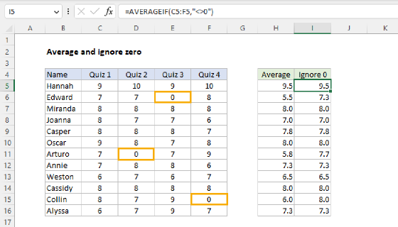
In the worksheet shown, this is the formula in cell E8. This works fine as long as the data contains only #N/A errors, but it will fail if there are other errors in the data. Another option with AVERAGEIF is to select only numbers that are greater than or equal to zero:
=AVERAGEIF(data,">=0") // zero or greater
This is the formula in E7. This simple formula works fine, as long as the numbers to average are not negative.
AGGREGATE
The simplest and most robust way to ignore errors when calculating an average is to use the AGGREGATE function. In cell E6, AGGREGATE is configured to average and ignore errors by setting function_num to 1, and options to 6:
=AGGREGATE(1,6,data) // average and ignore errors
This formula in E6 will ignore all errors that might appear in data, not just the #N/A error, and it will work fine with negative values. The AGGREGATE function is a "Swiss Army knife" function that can run other functions like SUM, COUNT, AVERAGE, MAX, etc. with special behaviors. For example, AGGREGATE can optionally ignore errors, hidden rows, and even other calculations. AGGREGATE can perform 19 different functions.
AVERAGE and IFERROR
It is possible to write an array formula that uses the AVERAGE function with the IFERROR function to filter out errors before averaging:
=AVERAGE(IFERROR(data,""))
Note: this is an array formula and must be entered with Control + Shift + Enter, except in Excel 365, where arrays are native.
IFERROR returns an alternative result when there is an error, and the original result when there is not. In this formula, the IFERROR function is used to catch errors in the data and convert them to empty strings (""). In the example shown, the named range data (B5:B15) contains eleven cells, which can be represented as an array like this:
{98;95;88;95;#N/A;75;90;100;#N/A;84;91} // 11 values in B5:B15
IFERROR converts the #N/A errors to empty strings ("") like this:
=IFERROR(data,"")
=IFERROR({98;95;88;95;#N/A;75;90;100;#N/A;84;91},"")
{98;95;88;95;"";75;90;100;"";84;91}
The resulting array is returned directly to the AVERAGE function:
=AVERAGE({98;95;88;95;"";75;90;100;"";84;91}) // returns 90.67
AVERAGE automatically ignores text values and returns the same result as above: 90.67.
AVERAGE and FILTER
Finally, in Excel 365, you can use the FILTER function together with the ISNUMBER function to filter out errors before they are averaged with a formula like this:
=AVERAGE(FILTER(data,ISNUMBER(data)))
Note: this is an array formula, but it only works in Excel 365, where arrays are native.
Here, the ISNUMBER function tests each value in data and returns an array of TRUE and FALSE values like this:
{TRUE;TRUE;TRUE;TRUE;FALSE;TRUE;TRUE;TRUE;FALSE;TRUE;TRUE}
Because there are 11 values in data, ISNUMBER returns 11 TRUE / FALSE results. TRUE corresponds to numeric values, and FALSE corresponds to non-numeric values. This array is returned directly to the FILTER function as the include argument:
FILTER(data,{TRUE;TRUE;TRUE;TRUE;FALSE;TRUE;TRUE;TRUE;FALSE;TRUE;TRUE})
FILTER then returns a "filtered array" that contains the 9 numeric values to AVERAGE:
=AVERAGE({98;95;88;95;75;90;100;84;91}) // returns 90.67
and AVERAGE returns 90.67.
Note: Be careful when ignoring errors. Suppressing errors can hide underlying problems.