Summary
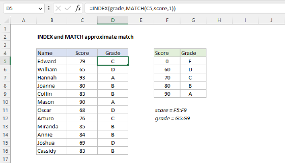
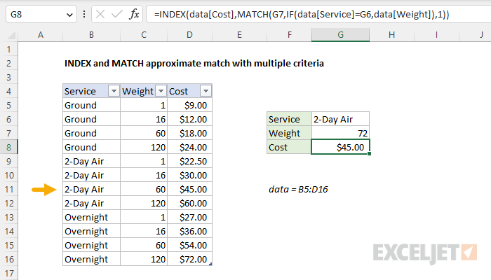
To perform an approximate match lookup with multiple criteria, you can use an INDEX and MATCH formula, with help from the IF function. In the example shown, the formula in G8 is:
=INDEX(data[Cost],MATCH(G7,IF(data[Service]=G6,data[Weight]),1))
where data is an Excel Table in the range B5:D16. With "2-Day Air" in cell G6 and 72 in cell G7, the formula returns $45.00.
Notes: (1) This is an array formula and must be entered with Control + Shift + Enter in older versions of Excel. (2) In the current version of Excel, you can use the same approach with an XLOOKUP formula.
Generic formula
=INDEX(range,MATCH(value,IF(range=A1,range),1))
Explanation
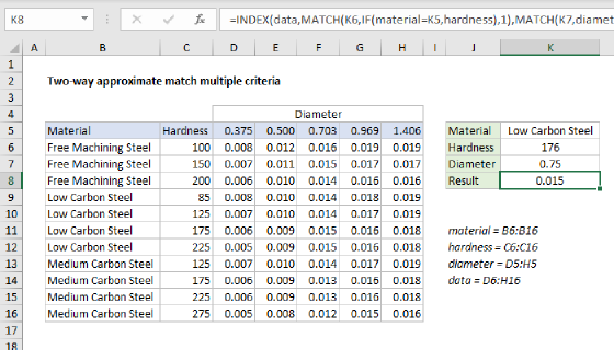
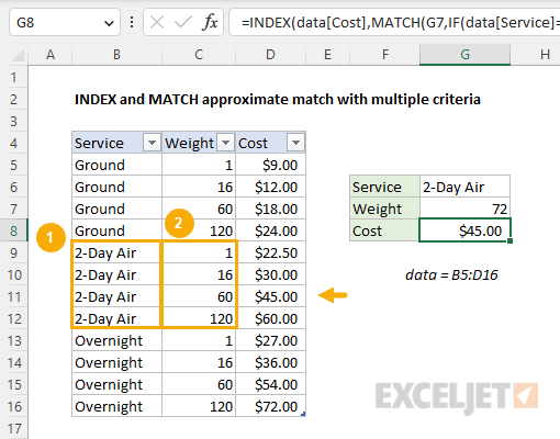
In this example, the goal is to look up the correct shipping cost for an item based on the shipping service selected and the item's weight. At the core, this is an approximate match lookup based on weight. The challenge is that we also need to filter by service. This means we must apply criteria in two steps: (1) match based on Service and (2) match based on Weight. The screen below shows the basic idea:
One way to solve this problem is with an INDEX and MATCH and the IF function to perform the required filtering. This works because the IF function returns 12 results, which map to the 12 rows in the table. This means MATCH will still return the correct row in the table even after IF has filtered out the other weights. See below for more details.
Background reading
This article assumes you are familiar with Excel Tables and INDEX and MATCH. If not, see:
- Excel Tables - introduction and overview
- How to use INDEX and MATCH - overview with simple examples
Basic INDEX and MATCH
In INDEX and MATCH formulas, the MATCH function finds the position of an item in a range, and the INDEX function returns the value at that position. If you are new to INDEX and MATCH, see this overview.
Looking at this example from the inside out, the core of the solution is an approximate match lookup based on weight. To illustrate, the screen below shows a simplified version of the same problem with the Service removed completely:
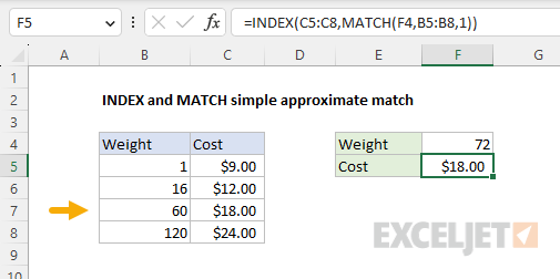
The formula in cell F5 is:
=INDEX(C5:C8,MATCH(F4,B5:B8,1))
Notice the match_type argument inside MATCH is set to 1, to locate the largest value in B5:B8 that is less than or equal to the lookup value in cell F4. In this case, the largest value less than or equal to 72 is 60, so MATCH returns 3 to INDEX as a row number, and INDEX returns $18.00 as a final result:
=INDEX(C5:C8,3) // returns 18
So far, so good. We have a simple working formula that returns the correct cost based on an approximate match lookup. The complication is that we also need to match based on Service. To do that, we need to extend the formula to handle multiple criteria.
Adding criteria for service
We know how to look up costs based on weight. The remaining challenge is that we also need to take into account Service. For simple exact-match scenarios, we can use Boolean logic, as explained here. But in this example, we need to perform an approximate match, so using Boolean logic will become complicated. Another approach is to "filter out" extraneous entries in the table so we are left only with entries that correspond to the Service we are looking up. The classic way to do this is with the IF function. This is the approach used in the example shown, where the formula in cell G8 is:
=INDEX(data[Cost],MATCH(G7,IF(data[Service]=G6,data[Weight]),1))
Note: this is an array formula and must be entered with Control + Shift + Enter in Legacy Excel.
The filtering is done with the IF function, which appears inside the MATCH function like this:
IF(data[Service]=G6,data[Weight])
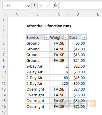
This code tests the values in the Service column to see if they match the value in G6. Where there is a match, the corresponding values in with Weight column are returned. If there is no match, the IF function returns FALSE. Because there are 12 rows in the table, the IF function returns an array that contains 12 results like this:
{FALSE;FALSE;FALSE;FALSE;1;16;60;120;FALSE;FALSE;FALSE;FALSE}
Notice the only weights that remain in the array are those that correspond to the "2-Day-Air" service; all other weights have been replaced with FALSE. You can visualize this operation in the original data like this:
This array is delivered directly to the MATCH function as the lookup_array:
MATCH(G7,{FALSE;FALSE;FALSE;FALSE;1;16;60;120;FALSE;FALSE;FALSE;FALSE},1)
The MATCH function then simply ignores the FALSE values and tries to match the remaining numbers. With a weight of 72 in cell G7, the MATCH function matches 60 and returns 7 to the INDEX function as row_num:
=INDEX(data[Cost],7) // returns 45
With a row number of 7, INDEX returns $45.00 as the final result.
Remember that we are using MATCH in an approximate match mode. With m**atch_type set to 1, values in the Weight column must be sorted in ascending order for MATCH to work correctly. See our MATCH function page for more information.