=RATE(nper, pmt, pv, [fv], [type], [guess])- nper - The total number of payment periods.
- pmt - The payment made each period.
- pv - The present value, or total value of all loan payments now.
- fv - [optional] The future value, or desired cash balance after last payment. Default is 0.
- type - [optional] When payments are due. 0 = end of period. 1 = beginning of period. Default is 0.
- guess - [optional] Your guess on the rate. Default is 10%.
Using the RATE function
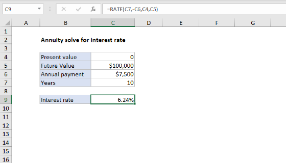
The RATE function returns the interest rate per period of an annuity. You can use RATE to calculate the periodic interest rate, then multiply as required to derive an annual interest rate. The RATE function is commonly multiplied by 12 to arrive at an annual rate.
The RATE function takes six arguments, the first three of which are required:
- nper (required) - The total number of payment periods in the annuity. For example, a 5-year car loan with monthly payments has 60 periods. You can enter nper as 5*12 to show how the number was determined.
- pmt (required) - The payment made each period. This number cannot change over the life of the annuity. In annuity functions, cash paid out is represented by a negative number. Note: If pmt is not provided, the optional fv argument must be supplied.
- pv (required) - The present value. This is the cash balance required after all payments have been made.
- fv (optional) - The future value, or a cash balance required after the last payment is made. When fv is omitted, it defaults to zero (0) and pmt must be provided.
- type (optional) - type is a boolean that controls when payments are due. Use 0 for payments due at the end of the period (regular annuities) and 1 for payments due at the beginning of the period (annuities due). Type defaults to 0 (end of period).
- guess (optional) - guess is a seed value to use for iteration. When omitted, guess defaults to 10%. Ordinarily, you can safely omit guess. If RATE does not converge, RATE will return a #NUM! error. Try different values for guess between 0 and 1.
RATE is calculated by iteration. If the results do not converge within 20 iterations, RATE returns a #NUM! error.
Example
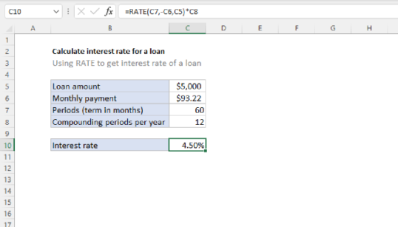
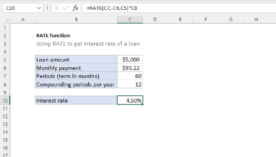
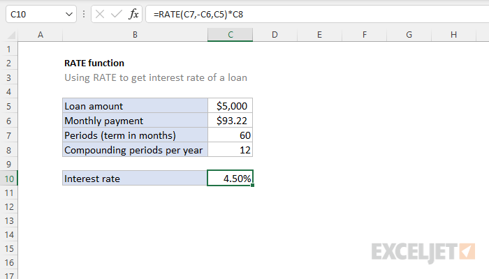
To calculate the annual interest rate for a $5000 loan with payments of $93.22 per month over 5 years, you can use RATE in a formula like this:
=RATE(60,-93.22,5000)*12 // returns 4.5%
In the example shown, the formula in C10 is:
=RATE(C7,-C6,C5)*C8 // returns 4.5%
Notice the value for pmt from C6 is entered as a negative value.
Use consistent values for guess and nper. If you make monthly payments on a five-year loan at 10 percent annual interest, use 10%/12 for guess and 5*12 for nper. If you make annual payments on the same loan, use 10% for guess and 5 for nper.
Notes
- The RATE formula is commonly multiplied by 12 to arrive at an annual rate.
- Be sure to use consistent values for guess and nper.