Summary
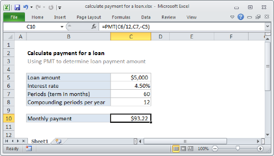
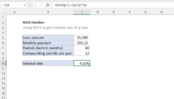
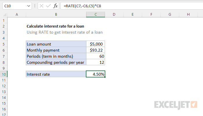
To calculate the periodic interest rate for a loan, given the loan amount, the number of payment periods, and the payment amount, you can use the RATE function. In the example shown, the formula in C10 is:
=RATE(C7,C6,-C5)*12
Generic formula
=RATE(periods,-payment,amount)*12
Explanation
Loans have four primary components: the amount, the interest rate, the number of periodic payments (the loan term) and a payment amount per period. One use of the RATE function is to calculate the periodic interest rate when the amount, number of payment periods, and payment amount are known.
In this example, we want to calculate the annual interest rate for 5-year, $5000 loan, and with monthly payments of $93.22. The RATE function is used like this:
=RATE(C7,-C6,C5)*C8
The function arguments are configured as follows:
nper - The number of periods is 60 (5 * 12), and comes from cell C7.
pmt - The payment is $93.22, and comes from cell C6. Note pmt is input as a negative value. In annuity functions, cash paid out is represented by a negative number. Note: If pmt is not provided, the optional fv argument must be supplied.
pv - The present value is $5000, and comes from C5.
With these inputs, the RATE function returns 0.375%, which is the periodic interest rate. To get an annual interest rate, we multiply by 12:
=RATE(C7,C6,-C5)*12
=0.003751*12
=0.0450
With the percent number format applied to cell C10, the result is displayed as 4.50%.