CUMPRINC Function

The CUMPRINC function calculates the cumulative principal amount paid over a specified range of time, defined by the start and end periods of a loan. This function is important for financial analysis, particularly in managing loans and amortization schedules. By calculating the principal portion of loan payments over specific periods, the CUMPRINC function provides useful insights into loan dynamics and helps show the trajectory of loan repayment over time. Typical use cases include evaluating the principal repayment structure of mortgages over various durations, analyzing the principal component in different loan offers, or planning financial budgets. 

Example

Assume a 5-year loan for $10,000 with an annual interest rate of 5%. Payments are monthly and there are 12 compounding periods per year. You want to confirm the total principal paid over the full term of the loan. You can calculate the total principal paid with the CUMPRINC function like this:

=CUMPRINC(5%/12,5*12,10000,1,5*12,0)

The inputs to CUMPRINC are as follows:

• rate = 5%/12 = 0.00416 (the annual interest rate divided by 12)
• nper = 5*12 = 60 (a 5-year loan has 60 periods)
• pv = 10,000 (the loan amount)
• start_period = 1 (the first period)
• end_period = 60 (the last period)
• type = 0 (payments at the end of each month)

The result is -10,000, which is the total principal paid over the full term of the loan. As expected, this is the original loan amount. The CUMPRINC returns a negative value because it represents an outflow of money. If you need a positive value, you can wrap the formula in the ABS function like this:

=ABS(CUMPRINC(5%/12,5*12,10000,1,5*12,0))

Worksheet example

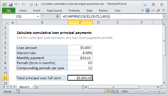
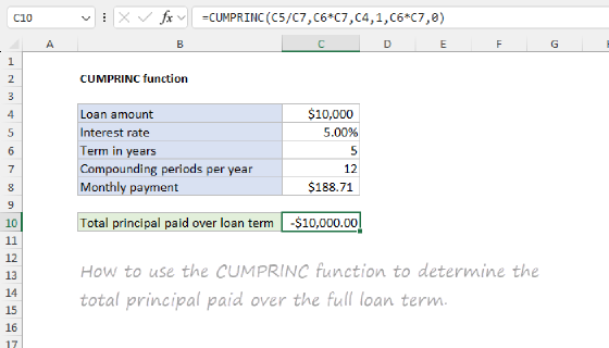
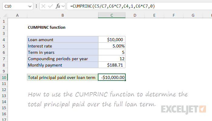
In the example above, all inputs to CUMPRINC are hardcoded to make the formula easier to read. In most cases, however, the main inputs will come from cell references. The screen below shows the same example can be set up in a worksheet:

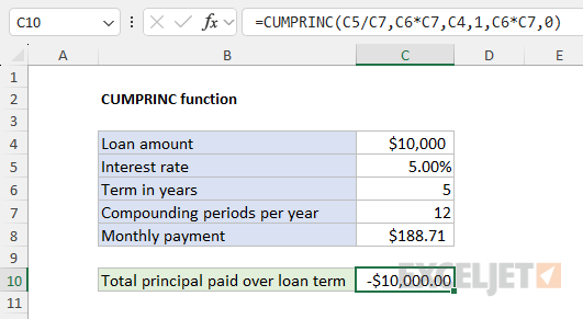
The formula in cell C10 is evaluated like this:

=CUMPRINC(C5/C7,C6*C7,C4,1,C6*C7,0)
=CUMPRINC(0.05/12,5*12,10000,1,5*12,0)
=CUMPRINC(0.0041667,60,10000,1,60,0)
=-10000

Notice that we provide the term as years * periods per year, instead of hardcoding the number 60 into the formula. Excel then calculates a value of 60 for nper before the CUMPRINC function runs. One reason to do it this way is to let Excel handle the math and provide a reminder of how we are deriving nper. More importantly, this also makes it possible for the formula to automatically adapt to a loan with a different term or a loan with a different number of compounding periods per year.

Also, notice that the monthly payment is not an input to CUMPRINC. This is because Excel can determine the regular payment amount based on the interest rate, number of periods, and principal amount. Excel calculates the interest due for a period and subtracts this amount from the payment to determine the principal payment.  To calculate a payment for a loan directly you can use the PMT function.

Notes

1. The interest rate can be provided as a percentage like 5% or a decimal number like 0.05.
2. Be consistent with inputs for rate. For example, for a 5-year loan with 6% annual interest, enter the rate as 6%/12.
3. The loan value (pv) must be entered as a positive value or CUMPRINC will return a #NUM! error.
4. The values for start_period and end_period should be integers between 1 and the total number of periods.
5. The value for start_period must be less than or equal to the value for end_period.