AVERAGEIF Function

The AVERAGEIF function calculates the average of the numbers in a range that meet supplied criteria. To apply criteria, the AVERAGEIF function supports logical operators (>,<,<>,=) and wildcards (*,?) for partial matching. AVERAGEIF can be used to average cells based on dates, numbers, and text. Note that AVERAGEIF only handles one condition. To apply multiple conditions, use the AVERAGEIFS function.

Caution - Unlike many Excel functions, *IFS functions like SUMIF, COUNTIF, and AVERAGEIF require actual cell ranges for their range arguments. They won't accept arrays created by functions like SEQUENCE, HSTACK, or FILTER. For example, this formula won't work:

=AVERAGEIF(SEQUENCE(10),">5") // won't work

Even though SEQUENCE(10) generates a list of numbers, it's not a valid range. This limitation wasn’t as noticeable before dynamic arrays, but it's more relevant now with newer Excel functions.

Syntax

The generic syntax for AVERAGEIF looks like this:

=AVERAGEIF(range,criteria,average_range)

The AVERAGEIF function takes three arguments: range, criteria, and average_range. Range is the range of cells to apply a condition to. Criteria is the condition to apply, along with any logical operators that are needed. Average_range argument is optional. When average_range is not provided, AVERAGEIF will average values in the range argument. When average_range is provided, AVERAGEIF will average values in average_range.  When using AVERAGEIF, keep the following in mind:

• AVERAGEIF will not include empty cells in the average, even when criteria match.
• AVERAGEIF will return a #DIV/0! error if no cells meet criteria.
• Criteria can include logical operators (>,<,<>,=) and wildcards (*,?) for partial matching.
• AVERAGEIF can only apply one criteria. To use multiple criteria, see the AVERAGEIFS function.

Criteria

The AVERAGEIF function supports logical operators (>,<,<>,=) and wildcards (*,?) for partial matching. Because AVERAGEIF is in a group of eight functions that split logical criteria into two parts, the syntax is a bit tricky. Range and criteria are provided separately, and operators in criteria need to be enclosed in double quotes (""). The table below shows some common examples:

Notice the last two examples use concatenation with the ampersand (&) character. When a criteria argument includes a value from another cell, or the result of a formula, logical operators like "<" must be joined with concatenation. This is because Excel needs to evaluate cell references and formulas first to get a value, before that value can be joined to an operator.

Examples

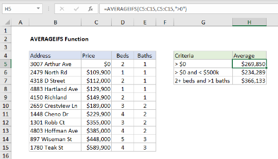
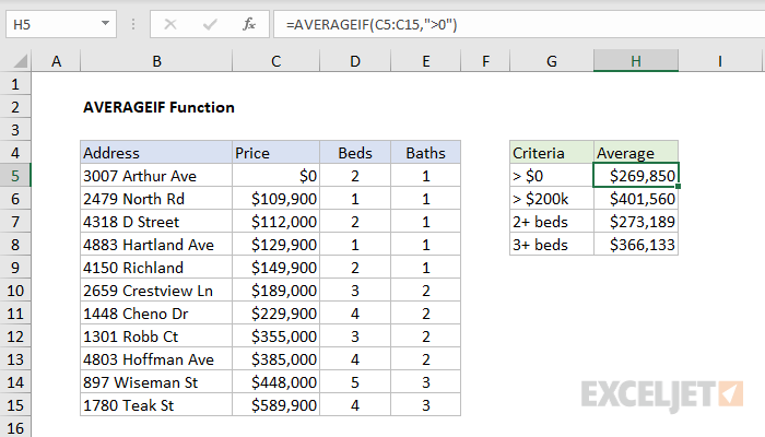
In the example shown the formulas in H5:H8 are as follows:

=AVERAGEIF(C5:C15,">0") // price greater than $0
=AVERAGEIF(C5:C15,">200000") // price greater than $200k
=AVERAGEIF(D5:D15,">=2",C5:C15) // 2+ bedrooms
=AVERAGEIF(D5:D15,">=3",C5:C15) // 3+ bedrooms

Double quotes ("") in criteria

In general, text values are enclosed in double quotes (""), and numbers are not. However, when a logical operator is included with a number, the number and operator must be enclosed in quotes. Note the difference in the two examples below. Because the second formula uses the greater than or equal to operator (>=), the operator and number are both enclosed in double quotes.

=AVERAGEIF(D5:D15,2,C5:C15) // 2 bedrooms
=AVERAGEIF(D5:D15,">=2",C5:C15) // 2+ bedrooms

Double quotes are also used for text values. For example, to average values in B1:B10 when values in A1:A10 equal "red", you can use a formula like this:

=AVERAGEIF(A1:A10,"red",B1:B10) // average "red" only

Value from another cell

A value from another cell can be included in criteria using concatenation. In the example below, AVERAGEIF will return the average of numbers in A1:A10 that are less than the value in cell B1. Notice the less than operator (which is text) is enclosed in quotes.

=AVERAGEIF(A1:A10,"<"&B1) // average values less than  B1

Wildcards

The wildcard characters question mark (?), asterisk(*), or tilde (~) can be used in criteria. A question mark (?) matches any one character and an asterisk (*) matches zero or more characters of any kind. For example, to average cells in a B1:B10 when cells in A1:A10 contain the text "red" anywhere, you can use a formula like this:

=AVERAGEIF(A1:A10,"*red*",B1:B10) // contains "red"

The tilde (~) is an escape character to allow you to find literal wildcards. For example, to match a literal question mark (?), asterisk(*), or tilde (~), add a tilde in front of the wildcard (i.e. ~?, ~*, ~~).

Average range caution

AVERAGEIF makes certain assumptions about the size of average_range, essentially resizing it when necessary to match the range argument, using the upper left cell in the range as an origin. In some cases, this behavior can create a result that seems reasonable but is in fact incorrect. For an example of this problem, see this article.

Notes

• TRUE and FALSE values ignored when calculating an average.
• Empty cells are ignored when calculating an average.
• AVERAGEIF returns #DIV/0! if no cells in range meet criteria.
• AVERAGEIF requires a range, you can't substitute an array.
• Average_range does not have to be the same size as range. The top left cell in average_range is used as the starting point, and cells that correspond to cells in range are averaged.
• AVERAGEIF supports wildcards but is not case-sensitive.