Explanation
In this example, the goal is to create automatic row numbers starting in cell B5 that match the data entered in column C. When new data is added to the list, the row numbers should increase as required. If items are deleted, the row numbers should respond accordingly. This has traditionally been a tricky problem in Excel because there is no built-in function to create and maintain row numbers. The article below explains several options. The best option for you will depend on what Excel version you use, and on your particular requirements.
Row numbers with the Fill Handle
The examples below use formulas to automatically generate row numbers. However, if you only need to enter row numbers on a one-time basis, you can use the fill handle to automate most of the process. The trick is to enter the first two numbers to help Excel understand what you want. Then select the two cells, and double click the fill handle to send it down, or simply drag the fill handle to the desired location. The animation below shows the basic process:

The advantage of this approach is you don't need to use any formulas at all. The disadvantage of this approach is that you will need to repeat the process if you add or remove items from the list, or if you otherwise want to generate a new set of row numbers.
Automatic row numbers with SEQUENCE
In the current version of Excel, the easiest way to create automatic row numbers is to use the SEQUENCE function. The SEQUENCE function generates a list of sequential numbers that spill directly on the worksheet. For example, to create numbers between 1-3 you can use SEQUENCE like this:
=SEQUENCE(3) // returns {1;2;3}
If you change rows to 5, SEQUENCE returns an array with 5 numbers:
=SEQUENCE(5) // returns {1;2;3;4;5}
The output from SEQUENCE is an array of values that will spill into multiple cells. The challenge in this example is how to calculate the number of rows needed for the list or table. We do this with the COUNTA function and a full column reference to column C like this:
=COUNTA(C:C) // returns 12
COUNTA returns 12, because there are 11 items in the list, plus the column header in cell C4. Because we are not assigning a row number to the header row, we need to subtract 1 to get a correct count:
=COUNTA(C:C)-1 // returns 11
Putting it all together, we have this formula in cell B5:
=SEQUENCE(COUNTA(C:C)-1)
Working from the inside out, COUNTA returns 12, from which 1 is subtracted, leaving 11:
=SEQUENCE(11)
SEQUENCE then returns an array that contains 11 numbers as a final result:
={1;2;3;4;5;6;7;8;9;10;11}
This array lands in cell B5 and spills into the range B5:B15. If the number of items in column C changes, COUNTA returns a new count, and SEQUENCE returns a new array of row numbers. Note that if there are other cells in column C that contain content that is not part of the data with row numbers, you have two choices. One option is to subtract a different number from COUNTA. For example, if there are two non-blank cells above the list in column C, you would subtract 2:
=SEQUENCE(COUNTA(C:C)-2)
Another option is to remove the full column range C:C and make the range more specific. For example:
=SEQUENCE(COUNTA(C5:C100))
Here the idea is that there will never be more than 100 items in the list, so we are only counting non-blank cells in the range C5:C100. This also means we will get a correct count from COUNTA with no need to subtract anything from the result.
Legacy Excel
In older versions of Excel that do not include the SEQUENCE function, you can use a more manual formula based on the ROW function. As the name implies, the ROW function returns the row number for a reference:
=ROW(A1) // returns 1
=ROW(E3) // returns 3
When a reference is not provided, ROW returns the row number of the cell the formula lives in. For example, if ROW is entered in cell B5, the result is 5:
=ROW() // returns 5 in B5
This means we can create sequential row numbers beginning with 1 by subtracting an appropriate offset value. For example to start numbering in cell B5, we can subtract 4 like this:
=ROW()-4 // returns 1 in B5
The catch with this formula is that you will need to manually copy it down column B to keep it in sync with the items in the list. This formula will continue to work as long as rows are not added or deleted above the first row of data. If rows are added or deleted above the data, or if you start the list in a different row, the hardcoded offset value 4 will need to be adjusted as needed.
Row numbers in an Excel Table
If you need to add automatic row numbers to an Excel Table, you can't use the SEQUENCE function, because Excel tables do not yet support dynamic array formulas. However, you can use a special formula based on the ROW function like this:
=ROW()-ROW(Table1[#Headers])
In this formula, the required offset is calculated based on the row number of the table header. In the worksheet shown, the header is in row 4. However, if the table exists at (or is moved to) another location, the formula will continue to work correctly.

See this article for a detailed explanation.
Row numbers for a named range
The approach for creating sequential row numbers in a table can be adapted to work with a named range like this:
=ROW()-ROW(INDEX(data,1,1))+1
Here, we are working with a single named range called data. To calculate the required offset, we use INDEX to get the location of the first cell in the range, then feed that result into the ROW function:
ROW(INDEX(data,1,1))
We pass the named range data into INDEX and request the cell at row 1, column 1. In other words, we are asking INDEX for the first (upper left) cell in the range. INDEX returns that cell as an address, and the ROW function returns the row number of that cell, which is used as the offset value explained above. The advantage of this formula is that it is portable. It won't break when the formula is moved, and it will work with any named range.
Related formulas

Add row numbers and skip blanks

Automatic row numbers in Table

Get relative row numbers in range

First row number in range
Add row numbers and skip blanks

Basic outline numbering

Last n rows
Related functions

SEQUENCE Function
The Excel SEQUENCE function generates a list of sequential numbers in an array. The array can be one dimensional, or two-dimensional, determined by rows and columns arguments. ...

ROW Function
The Excel ROW function returns the row number for a reference. For example, ROW(C5) returns 5, since C5 is the fifth row in the spreadsheet. When no reference is provided, ROW returns the row number of the cell which contains the formula.

INDEX Function
The Excel INDEX function returns the value at a given location in a range or array. You can use INDEX to retrieve individual values, or entire rows and columns. The MATCH function is often used together with INDEX to provide row and column numbers....

COUNTA Function
The Excel COUNTA function returns the count of cells that contain numbers, text, logical values, error values, and empty text (""). COUNTA does not count empty cells.
Related videos

The SEQUENCE function