Multiple cells have same value case sensitive

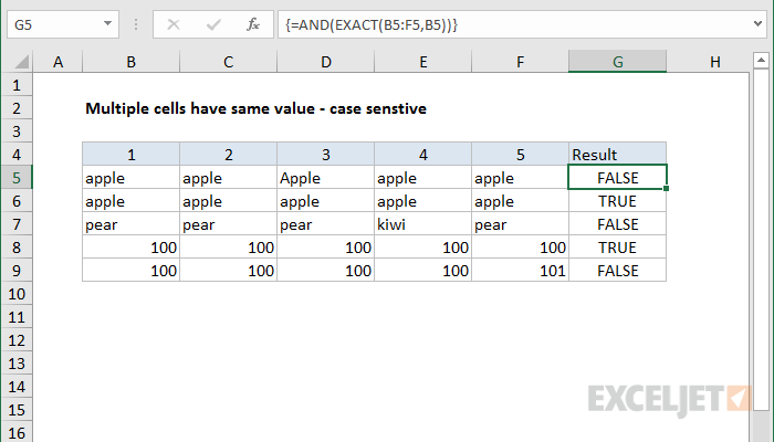
To verify that multiple cells have the same value with a case-sensitive formula, you can use a simple array formula based on the EXACT function with the AND function. In the example shown, the formula in G5 is:

=AND(EXACT(B5:F5,B5))

This is an array formula and must be entered with control + shift + enter

Explanation

This formula uses the EXACT formula to compare a range of cells to a single value:

=EXACT(B5:F5,B5)

Because we give EXACT a range of values in the first argument, we get back an array result containing TRUE FALSE values:

{TRUE,FALSE,TRUE,TRUE,TRUE}

This array goes into the AND function, which returns TRUE only if all values in the array are TRUE.

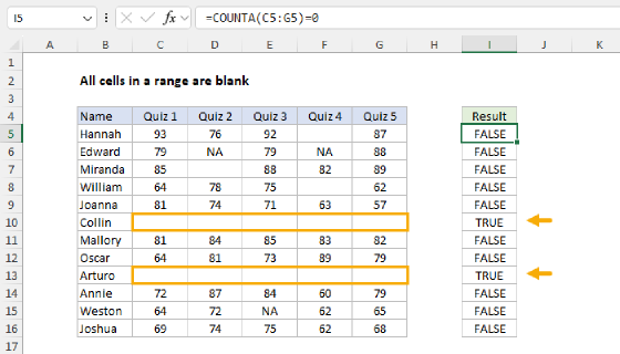
Ignore empty cells

To ignore empty cells, but still treat non-empty cells in a case-sensitive manner, you can use a version of the formula based on SUMPRODUCT:

=SUMPRODUCT(--(EXACT(range,value)))=COUNTA(range)

Here, we count exact matches using the same EXACT formula above, get a total count with SUMPRODUCT, and compare the result to a count of all non-empty cells, determined by COUNTA.

This is an array formula but control + shift + enter is not required because SUMPRODUCT handles the array natively.