Explanation
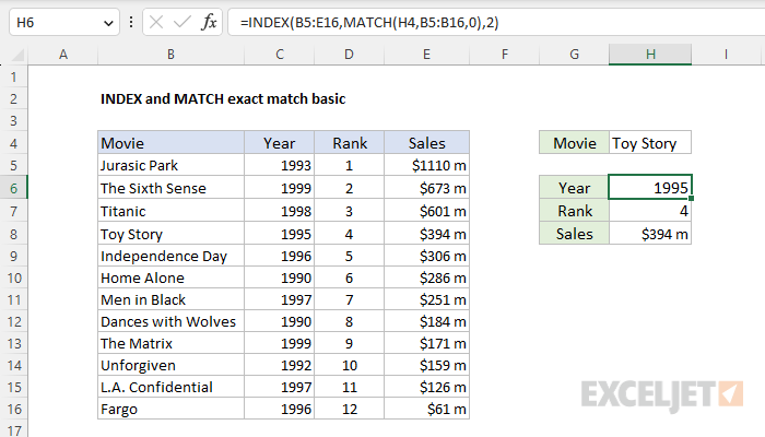
In this example, the goal is to look up various information about a random group of popular movies from the 1990s. The information to retrieve includes the year released, the rank against the other movies in the list, and worldwide gross sales. To retrieve this information, we are using an INDEX and MATCH formula that looks up information using the movie title. If you are new to INDEX and MATCH formulas, this article provides a detailed overview with many examples.
MATCH function
This formula uses the MATCH function to get the row position of Toy Story in the table, and the INDEX function to retrieve a value at that row. MATCH is configured to look for the movie title in cell H4 in the range B5:B16:
MATCH(H4,B5:B16,0)
Note that the match_type argument is set to zero (0), to force MATCH to perform an exact match. MATCH locates "Toy Story" on row 4 and returns this number to INDEX as the row number.
INDEX function
The INDEX function is configured with an array that includes all data in the table, and the column number is hard-coded as 2 to retrieve the Year value from column 2 in the table.
=INDEX(B5:E16,MATCH(H4,B5:B16,0),2) // get year
Once MATCH returns 4 to INDEX as the row number, we can simplify the formula to:
=INDEX(B5:E16,4,2) // returns 1995
INDEX then retrieves the value at the intersection of the 4th row and 2nd column in the array, which is 1995. The other formulas in the example are identical except for the column number:
=INDEX(B5:E16,MATCH(H4,B5:B16,0),2) // year
=INDEX(B5:E16,MATCH(H4,B5:B16,0),3) // rank
=INDEX(B5:E16,MATCH(H4,B5:B16,0),4) // sales
Note: normally, we would use absolute references to lock references like this:
=INDEX($B$5:$E$16,MATCH($H$4,$B$5:$B$16,0),2) // year
This will allow the formula to be copied into the range H6:H8 with these ranges locked. Then only the column number needs to be changed. However, in the examples above, we are using relative references to make the formulas easier to read.
INDEX with a single column
In the example above, INDEX receives an array that contains all data in the table. However, you can easily rewrite the formulas to provide INDEX with one column only, which eliminates the need to supply a column number:
=INDEX(C5:C16,MATCH(H4,B5:B16,0)) // year
=INDEX(D5:D16,MATCH(H4,B5:B16,0)) // rank
=INDEX(E5:E16,MATCH(H4,B5:B16,0)) // sales
In each case, INDEX receives a one-column array that corresponds to the data being retrieved, and MATCH supplies the row number.
INDEX with TRANSPOSE
The current version of Excel supports dynamic array formulas. This means a formula can return multiple values, and these values will spill onto the worksheet into multiple cells. This means it is possible to return the year, rank, and sales value all in one go. The trick is to give INDEX all 3 columns in the range C5:E16, then specify zero (0) for the row number:
INDEX(C5:E16,MATCH(H4,B5:B16,0),0)
Providing zero for the column_num argument will cause INDEX to return an entire row of data. With "Toy Story" in cell H4, we get back a horizontal array of values like this:
{1995,4,394436586} // {year,rank,sales}
This is the year, rank, and sales for Toy Story. To transform the horizontal data into a vertical array, we can nest the INDEX and MATCH formula inside the TRANSPOSE function like this:
=TRANSPOSE(INDEX(C5:E16,MATCH(H4,B5:B16,0),0))
The result is a vertical array that will land in cell H6 and spill into the range H6:H8 all in one step, with only one formula required.
How to use INDEX and MATCH - a detailed introduction with more examples


