Summary
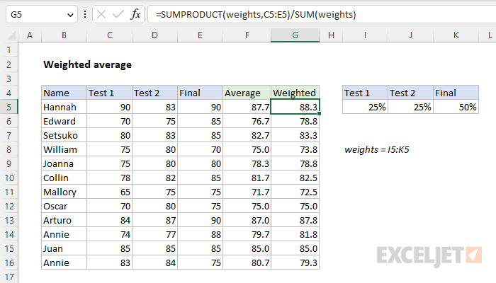
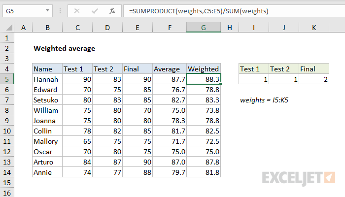
To calculated a weighted average, you can use a formula based on the SUMPRODUCT function and the SUM function. In the example shown, the formula in G5, copied down, is:
=SUMPRODUCT(weights,C5:E5)/SUM(weights)
where weights is the named range I5:K5. As the formula is copied down, it returns the weighted average seen in column G.
Generic formula
=SUMPRODUCT(weights,values)/SUM(weights)
Explanation
In this example, the goal is to calculate a weighted average of scores for each name in the table using the weights that appear in the named range weights (I5:K5) and the scores in columns C through E. A weighted average (also called a weighted mean) is an average where some values are more important than others. In other words, some values have more "weight". We can calculate a weighted average by multiplying the values to average by their corresponding weights, then dividing the sum of results by the sum of weights. In Excel, this can be represented with the generic formula below, where weights and values are cell ranges:
=SUMPRODUCT(weights,values)/SUM(weights)
The core of this formula is the SUMPRODUCT function. In a nutshell, SUMPRODUCT multiplies ranges or arrays together and returns the sum of products. This sounds really boring, but SUMPRODUCT is an incredibly versatile function that shows up in all kinds of useful formulas. See this page for an overview.
Worksheet example
In the worksheet shown, scores for 3 tests appear in columns C through E, and weights appear in the named range weights (I5:K5). The formula in cell G5 is:
=SUMPRODUCT(weights,C5:E5)/SUM(weights)
Looking first at the left side, we use the SUMPRODUCT function to multiply weights by corresponding scores and sum the result:
=SUMPRODUCT(weights,C5:E5) // returns 88.25
SUMPRODUCT multiplies corresponding elements of the two arrays together, then returns the sum of the product. We can visualize this operation in cell G5 like this:
=SUMPRODUCT({0.25,0.25,0.5},{90,83,90})
=SUMPRODUCT({22.5,20.75,45})
=88.25
The result is then divided by the sum of the weights:
=88.25/SUM(weights)
=88.25/SUM({0.25,0.25,0.5})
=88.25/1
=88.25
Note: when calculating a weighted average, it is common to assign weights that add up to the number 1. As you can see above, when the weights do add up to 1, the denominator becomes 1 and has no effect in the formula. However, it is not required that weights add up to 1, and the general form of the formula used above is meant to handle either case. See below for an example where weights do not add up to 1.
As the formula is copied down column G, the named range weights I5:K5 does not change, since it behaves like an absolute reference. However, the scores in C5:E5, which are relative reference, change with each new row. The result is a weighted average for each name in the list as shown. For easy reference, the average in column F is calculated normally with the AVERAGE function:
=AVERAGE(C5:E5)
Weights that do not sum to 1
In the example above, the weights are configured to add up to 1, so the divisor is 1, and the final result is the value returned by SUMPRODUCT. However, a nice feature of the formula is that the weights don't need to add up to 1. For example, we could use a weight of 1 for the first two tests and a weight of 2 for the final (since the final is twice as important) and the weighted average will be the same:
In cell G5, the formula is solved like this:
=SUMPRODUCT(weights,C5:E5)/SUM(weights)
=SUMPRODUCT({1,1,2},{90,83,90})/SUM(1,1,2)
=SUMPRODUCT({90,83,180})/SUM(1,1,2)
=353/4
=88.25
Note: the values in curly braces {} above are arrays, which map directly to ranges in Excel.
Transposing weights
The SUMPRODUCT function requires that array dimensions be compatible to run correctly. For example, if the data is in a horizontal array, the weights should also be in a horizontal array. If dimensions are not compatible, SUMPRODUCT will return a #VALUE error. To prevent this problem, you may need to transpose the weights to match the data. In the example below, the weights are the same as the original example above, but they are listed in a vertical range:
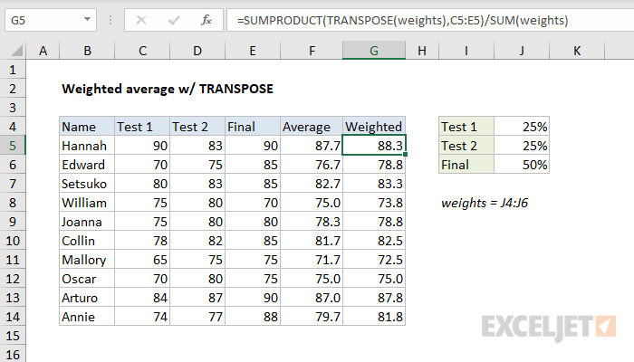
In this case, to calculate a weighted average with the same formula, we need to "flip" the weights into a horizontal array with the TRANSPOSE function like this:
=SUMPRODUCT(TRANSPOSE(weights),C5:E5)/SUM(weights)
After TRANSPOSE runs, the vertical array:
=TRANSPOSE({0.25;0.25;0.5}) // vertical array
becomes a horizontal array like this:
={0.25,0.25,0.5} // horizontal array
Note the semicolons are now commas, which indicate a horizontal array. From this point, the formula is solved the same way as explained earlier.
Video: What is an array?