Summary
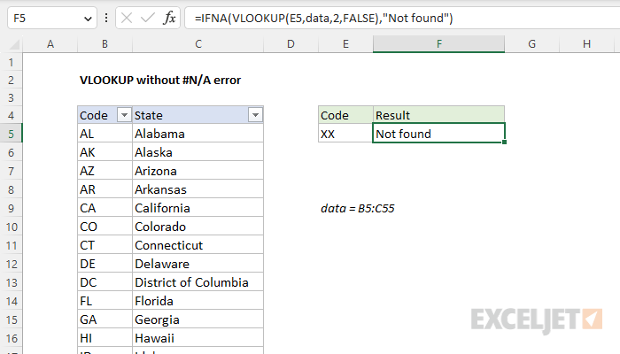
To hide the #N/A error that VLOOKUP returns when it can't find a lookup value, you can use the IFNA function to catch the error and return any value you like. In the example shown, the formula in cell F5 is:
=IFNA(VLOOKUP(E5,data,2,FALSE),"Not found")
where data is an Excel Table in the range B5:C55. The result is "Not Found" because "XX" does not exist in the Code column. When a valid 2-letter code is entered in cell E5, VLOOKUP will function normally. For example, if "GA" is entered in cell E5, VLOOKUP will return "Georgia":
Generic formula
=IFNA(VLOOKUP(value,table,column,FALSE),"message")
Explanation
When VLOOKUP can't find a value in a lookup table, it returns the #N/A error. In this example, the goal is to remove the #N/A error that VLOOKUP returns when it can't find a lookup value. In general, the best way to do this is to use the IFNA function. However, the IFERROR function can also be used in the same way. Both options are explained below.
VLOOKUP function
The VLOOKUP function performs a lookup operation on vertical data. The generic syntax for VLOOKUP looks like this:
VLOOKUP(A1,table,column,FALSE)
Where A1 contains a value to lookup, table is the data, column is a number, and FALSE specifies exact match, which is required in this example. In the workbook shown, we want to enter an abbreviation in cell E5 and get the correct State name in cell F5, where all data is in an Excel Table named data. To do this, we can use VLOOKUP in a formula like this:
VLOOKUP(E5,data,2,FALSE)
When a valid 2-letter code is entered in cell E5, VLOOKUP will return the corresponding State. For example, if "CA" is entered in cell E5, VLOOKUP will return "California":
VLOOKUP("CA",data,2,FALSE) // returns "California"
If an invalid code is entered in cell E5, VLOOKUP will return an #N/A error:
VLOOKUP("XX",data,2,FALSE) // returns #N/A
The screen below shows how this error looks on the worksheet:
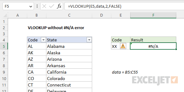
The #N/A error technically means "not available". However, you may want to return a more friendly result. You can do this by combining VLOOKUP with the IFNA function.
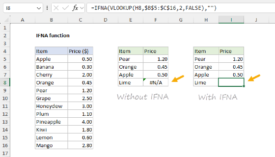
VLOOKUP with IFNA
The IFNA function is a simple way to trap and handle #N/A errors without catching other errors. When used with a formula, the generic syntax looks like this:
=IFNA(formula,alternative)
Here, the formula might return a #N/A error; the alternative is the value or formula to return in that case. To trap the #N/A error in this example, we wrap the IFNA function around the original VLOOKUP function and provide an alternate value. For example, to return "Not found" when VLOOKUP returns #N/A, we can use a formula like this:
=IFNA(VLOOKUP(E5,data,2,FALSE),"Not found")
Now, when VLOOKUP returns the #N/A error, IFNA takes over and returns "Not found":
=IFNA(VLOOKUP("XX",data,2,FALSE),"Not found") // returns "Not found"
To return a different message, just change the second argument in IFNA:
=IFNA(VLOOKUP("XX",data,2,FALSE),"Invalid code") // returns "Invalid code"
If you would prefer to return nothing, you can provide an empty string ("") instead, like this:
=IFNA(VLOOKUP("XX",data,2,FALSE),"") // returns ""
The result from this formula will look like an empty cell when the lookup Code is not found.
VLOOKUP with IFERROR
You can also trap #N/A errors returned by VLOOKUP with the IFERROR function like this:
=IFERROR(VLOOKUP(E5,data,2,FALSE),"Not found")
IFERROR works just like the IFNA function — it catches an #N/A error returned by VLOOKUP and returns an alternative result. The difference is that IFERROR will catch other errors as well.
The #N/A error is Excel's way of telling you a value was not found. With the more general IFERROR function, there is a risk that you might catch other unrelated errors and return a confusing result. For example, if you have a typo in a function name, Excel will return a #NAME! error. Or, if rows/columns are deleted in a worksheet, a formula may return a #REF! error. While IFNA will let these errors come through (so you see them), IFERROR will catch these errors, too, which can hide the underlying problem. For these reasons, I recommend you use the IFNA function when the purpose is to trap #N/A errors only.
Older versions of Excel
In earlier versions of Excel that lack the IFNA function, you will need to repeat the VLOOKUP inside an IF function that catches an error with the ISNA function. For example:
=IF(ISNA(VLOOKUP(A1,table,2,FALSE)),"Not found",VLOOKUP(A1,table,2,FALSE))