Summary
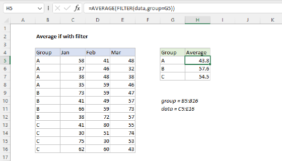
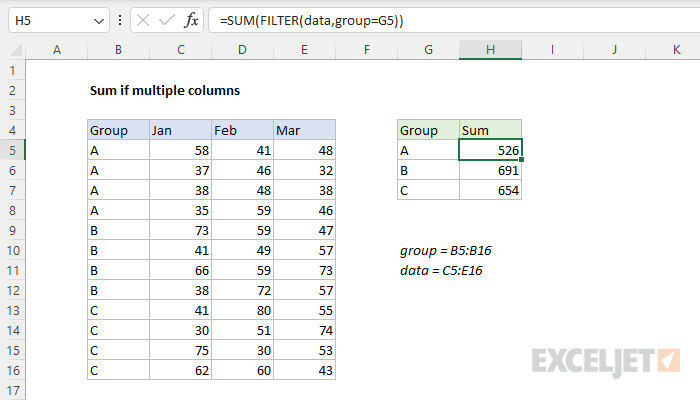
To calculate a conditional sum for multiple columns of data, you can use a formula based on SUM function and the FILTER function. In the example shown, the formula in H5, copied down, is:
=SUM(FILTER(data,group=G5))
Here, data (C5:E16) and group (B5:B16) are named ranges. The result is the sum of values in group "A" for all three months of data. As the formula is copied down, it calculates a sum for each group in column G.
The FILTER function is only available in Excel 2021 or later. See below for a formula based on SUMPRODUCT that will work in all versions of Excel.
Generic formula
=SUM(FILTER(data,criteria))
Explanation
In this example, the goal is to calculate a sum for any given group ("A", "B", or "C") across all three months of data in the range C5:E16. In other words, we want to perform a "sum if" with a data range that contains three columns. For convenience only, data (C5:E16) and group (B5:B16) are named ranges. The article below covers the following topics:
- Why SUMIFS won't work
- FILTER solution
- SUMPRODUCT solution
- More advanced criteria
- Clever all-in-one-formula
In Excel 2021 or later, the FILTER solution is easy and intuitive. If you are using an older version of Excel, use the SUMPRODUCT option. The section on advanced criteria covers both options.
Why SUMIFS won't work
You might be tempted to solve this problem with the SUMIFS function or the SUMIF function. After all, it seems simple enough - we need to check if group (B5:B16) is equal to "A" or "B" or "C", then sum the corresponding numbers in columns C, D, and E. In fact, we can easily use SUMIFS to calculate a sum for a given group on one month of data. For example, to calculate a sum for group "A" in January, we can use a formula like this:
=SUMIFS(C5:C16,group,"A") // returns 168
However, if you try to expand sum_range to include all three columns in data (C5:E16), you'll get a #VALUE! error:
=SUMIFS(data,group,"A") // returns #VALUE!
Why? The reason is that SUMIFS expects sum_range to be the same size as criteria_range. When we try to use the 1-column range group (B5:B16) with the 3-column range data (C5:E16), SUMIFS returns an error. What about the SUMIF function? If we give the older SUMIF function the entire data range and the same criteria, we don't get an error, but we do get an incorrect result:
=SUMIF(group,"A",data) // returns 168
This happens because SUMIF assumes that the sum_range is the same size as the range. Basically, SUMIF resizes sum_range to match the range argument. This kind of "silent failure" is dangerous because the result seems reasonable but is, in fact, incorrect. You may not like formula errors, but at least they tell you something is wrong!
So, at this point, we could start chaining together multiple SUMIF or SUMIFS functions like this:
=SUMIFS(C5:C16,group,"A")+SUMIFS(D5:D16,group,"A")+SUMIFS(E5:E16,group,"A")
But there must be a better way to do this in Excel, right? Yes!
FILTER solution
In the current version of Excel, a nice solution is the SUM function with the FILTER function. This is the approach used in the worksheet shown, where the formula in cell H5, copied down, is:
=SUM(FILTER(data,group=G5))
Where data (C5:E16) and group (B5:B16) are named ranges. Inside the SUM function, the FILTER function is configured to filter the data in C5:E16 with a simple logical expression:
FILTER(data,group=G5)
Because cell G5 contains "A", and group (B5:B16) contains 12 values, the expression returns an array with 12 TRUE and FALSE values like this:
{TRUE;TRUE;TRUE;TRUE;FALSE;FALSE;FALSE;FALSE;FALSE;FALSE;FALSE;FALSE}
Notice the first four values in the array are TRUE, which corresponds to the first 4 rows in the data, which are in group A. This array is returned to the FILTER function as the include argument, and FILTER uses this array to select the first 4 rows of data (C5:E16).
The result from FILTER is delivered directly to the SUM function as a single array:
=SUM({58,41,48;37,46,32;38,48,38;35,59,46})
SUM returns a final result of 526, the sum of the 12 numbers in the array returned by FILTER. As the formula is copied down, it calculates the correct sum for each group.
This is a good example of how the FILTER function can change how you think about a problem in Excel. The trick is realizing that you can solve the problem in two simple steps: (1) filter the data, then (2) sum the data. If you are new to the FILTER function, see this short video for a quick intro.
SUMPRODUCT solution
You can use the SUMPRODUCT function to solve this problem in older versions of Excel like this:
=SUMPRODUCT(--(group=G5)*data)
Working from the inside out, the logical expression on the left tests for group A like this:
--(group=G5) // test all group values
Since we are comparing one value in G5 to the 12 values in group, we get back 12 results:
--{TRUE;TRUE;TRUE;TRUE;FALSE;FALSE;FALSE;FALSE;FALSE;FALSE;FALSE;FALSE}
Next, we use a double-negative (--) to convert the TRUE and FALSE values to 1s and 0s. At this point, the result inside of SUMPRODUCT looks like this:
=SUMPRODUCT({1;1;1;1;0;0;0;0;0;0;0;0}*data)
Notes: (1) technically, the double negative (--) is unnecessary in this formula because multiplying the TRUE and FALSE values by the numeric values in the data will automatically convert TRUE and FALSE values to 1s and 0s. However, the double negative does no harm, and I think it makes the formula easier to understand because it signals a Boolean operation. (2) Like SUMIFS, SUMPRODUCT also requires that range/array arguments be the same size. We side-step this requirement above by multiplying the group * data inside array1. The result is that SUMPRODUCT only gets a single array.
After multiplication, we have a single array in SUMPRODUCT like this:
=SUMPRODUCT({58,41,48;37,46,32;38,48,38;35,59,46;0,0,0;0,0,0;0,0,0;0,0,0;0,0,0;0,0,0;0,0,0;0,0,0})
Notice the Boolean array acts like a filter to "cancel out" values not associated with group "A". Only the 12 values in group A survive the operation, while the other 24 values are forced to zero. With just a single array to process, SUMPRODUCT sums the array and returns a final result: 526.
Note: although this is an array formula, the SUMPRODUCT formula does not need to be entered in a special way with control + shift + enter, because SUMPRODUCT can handle array operations natively.
More advanced criteria
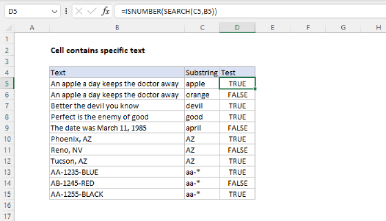
Although the criteria needed for this example is simple (test for a specific group), you can adapt the criteria to handle more complex scenarios. For example, to perform a "contains" type search for a substring, you could use a FILTER formula like this:
=SUM(FILTER(data,ISNUMBER(SEARCH(G5,group))))
Or a SUMPRODUCT formula like this:
=SUMPRODUCT(--ISNUMBER(SEARCH(G5,group))*data)
These formulas will sum by group, treating the value in G5 as a substring. For more information about this particular logic, see this example.
Clever all-in-one formula
In the latest version of Excel 365, you can solve this problem with a clever all-in-one formula based on the GROUPBY function and the BYROW function. In the workbook below, there is just one formula entered in cell G5:
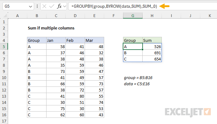
In this formula, the BROW function generates a sum for each row in "data", and the GROUPBY function groups these sums by the group values in column C automatically. Pretty cool!