Summary
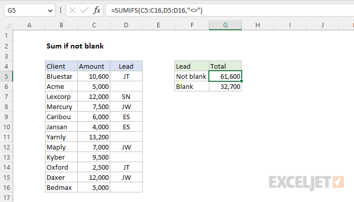
To sum values when corresponding cells are not blank, you can use the SUMIFS function. In the example shown, the formula in cell G5 is:
=SUMIFS(C5:C16,D5:D16,"<>")
The result is 61,600, the sum of amounts in C5:C16 when corresponding cells in D5:D16 are not blank.
Generic formula
=SUMIFS(sum_range,range,"<>")
Explanation
In this example, the goal is to sum the Amounts in C5:C16 when the Lead in D5:D16 is not blank (i.e., not empty). A good way to solve this problem is to use the SUMIFS function. However, you can also use the SUMPRODUCT function or the FILTER function, as explained below. Because SUMPRODUCT and FILTER can work with ranges and arrays, they are more flexible.
Background study
SUMIFS Function
The SUMIFS function sums cells in a range that meet one or more conditions, referred to as criteria. To apply criteria, the SUMIFS function supports logical operators (>,<,<>,=) and wildcards (*,?) for partial matching. The generic syntax for SUMIFS with one condition looks like this:
=SUMIFS(sum_range,range1,criteria1) // 1 condition
In this case, we need to test for only one condition, which is that the cells in D5:D16 are not blank. We start off with the sum_range, which contains the amounts in C5:C16:
=SUMIFS(C5:C16,
Next, we add the range that we need to test, which in D5:D16:
=SUMIFS(C5:C16,D5:D16,
Finally, we add the criteria, which is not equal to operator (<>), which must be enclosed in double quotes (""):
=SUMIFS(C5:C16,D5:D16,"<>")
The result is 61,600, the sum of amounts in C5:C16 when corresponding cells in D5:D16 are not blank. The main challenge with SUMIFS is the quirky syntax. For criteria, we simply use the "not equal to" operator, "<>". We don't provide a value, and it's implied that this means "not equal to nothing", i.e., "not blank". To read more about how to use the SUMIFS function with logical operators and wildcards, see this page.
SUMPRODUCT function
Another way to solve this problem is with the SUMPRODUCT function and a formula like this:
=SUMPRODUCT((D5:D16<>"")*C5:C16)
This is an example of using Boolean logic in Excel. The expression on the left checks if the cells in D5:D16 are not empty:
(D5:D16<>"")
Because there are 12 cells in D5:D16, the expression returns an array of 12 TRUE and FALSE values:
{TRUE;FALSE;TRUE;TRUE;TRUE;TRUE;FALSE;TRUE;FALSE;TRUE;TRUE;FALSE}
Note the TRUE values correspond to cells in D5:D16 that are not blank. Next, the math operation of multiplying this array by the range numeric values in C5:C16 automatically converts the TRUE and FALSE values to an array of 1s and 0s. Inside SUMPRODUCT, we can visualize the operation like this:
=SUMPRODUCT({1;0;1;1;1;1;0;1;0;1;1;0}*C5:C16)
In this form, you can see how the logic works. When the Boolean array is multiplied by C5:C16, it acts like a filter that only allows values associated with 1s to pass through; other values are "zeroed out". After multiplication, we have one array:
=SUMPRODUCT({10600;0;12000;7500;6000;4000;0;7000;0;2500;12000;0})
With only one array to process, SUMPRODUCT sums the array and returns 61,600 as a final result. One advantage of SUMPRODUCT is that it can handle array operations natively. This can be handy when you want to adjust a formula to use more specific logic that is not supported by SUMIFS. For more information, see Why SUMPRODUCT?
FILTER function
In the latest version of Excel, another approach is to use the FILTER function with the SUM function in a formula like this:
=SUM(FILTER(C5:C16,D5:D16<>"",0))
In this formula, we are literally removing values we don't want to sum. The FILTER function is configured to return only values in C5:C16 when cells in D5:D16 are not empty. The result inside SUM looks like this:
=SUM({10600;12000;7500;6000;4000;7000;2500;12000})
The final result is 61,600. Like SUMPRODUCT, FILTER is a more flexible function that can apply criteria in ways that SUMIFS can't. For more on the FILTER function, see this page.
Sum if blank
The formulas above can be easily adjusted to sum amounts when corresponding cells in D5:D16 are blank. In the worksheet shown, the formula in cell G6 is:
=SUMIFS(C5:C16,D5:D16,"")
The result is 32,700, the sum of amounts in C5:C16 when corresponding cells in D5:D16 are blank. The equivalent SUMPRODUCT and FILTER formulas are as follows:
=SUMPRODUCT((D5:D16="")*C5:C16)
=SUM(FILTER(C5:C16,D5:D16="",0))
These formulas also return 32,700.