Summary
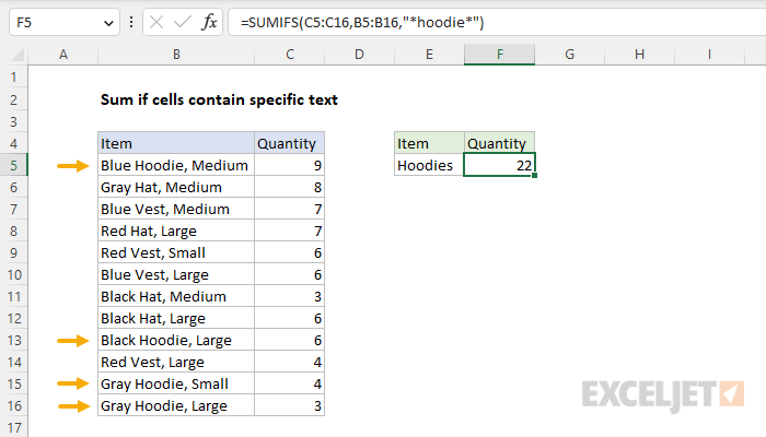
To sum if cells contain specific text, you can use the SUMIFS or SUMIF function with a wildcard. In the example shown, the formula in cell F5 is:
=SUMIFS(C5:C16,B5:B16,"*hoodie*")
This formula sums the quantity in column C when the text in column B contains "hoodie". Note that SUMIFS is not case-sensitive. However, see below for a case-sensitive option.
Generic formula
=SUMIFS(sum_range,range,"*text*")
Explanation
In this example, the goal is to sum the quantities in column C when the text in column B contains "hoodie". The challenge is that the item names ("Hoodie", "Vest", "Hat") are embedded in a text string that also contains size and color. This means we need to apply criteria that looks for a substring in the item text. To solve this problem, you can use either the SUMIFS function or the SUMIF function with a wildcard. If you need a case-sensitive formula, you can use the SUMPRODUCT function with the FIND function. All three approaches are explained below.
Note: this example embeds wildcards together with the search substring to keep things simple. However, you can also use wildcards with text in another cell, as explained in this more advanced example.
Wildcards
Excel functions like SUMIF and SUMIFS support the wildcard characters "?" (any one character) and "" (zero or more characters), which can be used in criteria. Wildcards allow you to create criteria to target cells that "begin with", "end with", "contain 3 characters" and so on. The table below shows some examples. For this problem, we want to use the "Cells that contain text in xyz" pattern, which uses two asterisks (), one before and one after the search string like this "xyz".
| Target | Criteria |
|---|---|
| Cells with 3 characters | "???" |
| Cells equal to "xyz", "xaz", "xbz", etc | "x?z" |
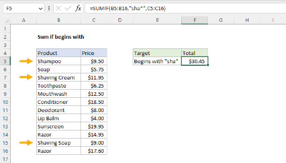
| Cells that begin with "xyz" | "xyz*" |
| Cells that end with "xyz" | "*xyz" |
| Cells that contain "xyz" | "xyz" |
| Cells that contain text in A1 | ""&A1&"" |
Note that wildcards are enclosed in double quotes ("") when they appear in criteria.
SUMIFS solution
One way to solve this problem is with the SUMIFS function. SUMIFS can handle multiple criteria, and the generic syntax for a single condition looks like this:
=SUMIFS(sum_range,criteria_range1,criteria1)
Notice that the sum range always comes first in the SUMIFS function. In our case, the sum_range is C5:C16, criteria_range1 is B5:B16, and criteria1 is "hoodie". Putting it all together, the formula in cell F5 of the worksheet shown is:
=SUMIFS(C5:C16,B5:B16,"*hoodie*")
Notice the text and both wildcards (*) are enclosed in double quotes (""). The meaning of this criteria is to match the substring "hoodie" anywhere in a text string. When the formula is entered in cell F5, it returns 22, the total quantity of "hoodie" products in the data.
SUMIF solution
This problem can also be solved with the SUMIF function, where the equivalent formula is:
=SUMIF(B5:B16,"*hoodie*",C5:C16)
Note that sum_range is the last argument in the SUMIF function. However, the criteria itself is identical to what we used in SUMIFS above. The result returned by SUMIF is also the same: 22.
Case-sensitive option
As mentioned above, the SUMIF and SUMIFS functions are not case-sensitive. If you need a case-sensitive solution, you can use a formula based on the SUMPRODUCT function and the FIND function like this:
=SUMPRODUCT(--ISNUMBER(FIND("Hoodie",B5:B16))*C5:C16)
Inside SUMPRODUCT, the left side of the expression tests for "Hoodie" with ISNUMBER and FIND:
--ISNUMBER(FIND("Hoodie",B5:B16))
Note the "H" in hoodie is capitalized. The FIND function is always case-sensitive, and returns the position of find_text as a number when found, and a #VALUE! error when not found. We do not need to use a wildcard like (*) because FIND automatically searches for a substring. Because there are 12 values in B5:B16, FIND returns an array of 12 results like this:
{6;#VALUE!;#VALUE!;#VALUE!;#VALUE!;#VALUE!;#VALUE!;#VALUE!;7;#VALUE!;6;6}
Notice that FIND returns numbers for rows 1, 9, 11, and 12 in the data. These are the rows where the substring "Hoodie" appears in the text. Next, the ISNUMBER function converts the results from FIND into TRUE and FALSE values, and the double negative (--) converts the TRUE and FALSE values to 1s and 0s. Inside SUMPRODUCT we now have:
=SUMPRODUCT({1;0;0;0;0;0;0;0;1;0;1;1}*C5:C16)
Note: technically, the double negative (--) is unnecessary in this formula, because multiplying the TRUE and FALSE values by the numeric values in C5:C16 will automatically convert TRUE and FALSE values to 1s and 0s. However, the double negative does no harm and it makes the formula a bit easier to understand, because it indicates a Boolean operation.
When the two arrays are multiplied together, the zeros in the first array work like a filter to "cancel out" the quantity for items that are not "Hoodies". The result inside SUMPRODUCT is a single array like this:
=SUMPRODUCT({9;0;0;0;0;0;0;0;6;0;4;3})
With only one array to process, SUMPRODUCT sums the array and returns 22 as a final result. For a more detailed explanation of FIND + ISNUMBER see this article. To adapt this formula to use text in cell references, see this example.
Note: In Excel 365, you can replace SUMPRODUCT with the SUM function. To read more about this, see Why SUMPRODUCT?