Summary
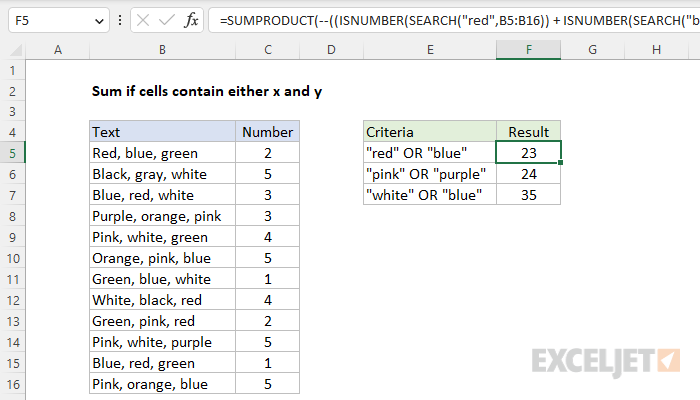
To sum cells that contain either x or y as substrings, you can use the SUMPRODUCT function together with ISNUMBER and SEARCH. In the example shown, the formula in cell F5 is:
=SUMPRODUCT(--((ISNUMBER(SEARCH("red",B5:B16)) + ISNUMBER(SEARCH("blue",B5:B16)))>0),C5:C16)
The result is 23, the sum of numbers in C5:C16 when text in B5:B16 contains the substring "red" or the substring "blue".
Generic formula
=SUMPRODUCT(--((ISNUMBER(SEARCH("red",range1)) + ISNUMBER(SEARCH("blue",range1)))>0),range2)
Explanation
In this example, the goal is to sum numbers in the range C5:C16 when text in the range B5:B16 contains the substring "red" OR the substring "blue". In other words, if the text in B5:B16 contains either of these two text values in any location, the corresponding number in C5:C16 should be included in the sum. We can't use the SUMIFS function with two criteria because SUMIFS is based on AND logic, and both criteria would need to be TRUE. And if we try to use two SUMIFS formulas (i.e., SUMIFS + SUMIFS), we will double count some numbers because some cells in B5:B16 contain both "red" and "blue". One solution is to use the SUMPRODUCT function together with the ISNUMBER and SEARCH functions.
SEARCH + ISNUMBER for substrings
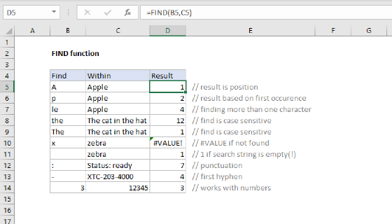
The core of this formula is based on the SEARCH function together with the ISNUMBER function. The SEARCH function is designed to find a specific substring in a text string. If SEARCH finds the substring, it returns the position of the substring in the text as a number. If the substring is not found, SEARCH returns a #VALUE error. For example:
=SEARCH("p","apple") // returns 2
=SEARCH("z","apple") // returns #VALUE!
To force a TRUE or FALSE result, we can use the ISNUMBER function. ISNUMBER returns TRUE for numeric values and FALSE for anything else. So, if SEARCH finds the substring, it returns the position as a number, and ISNUMBER returns TRUE:
=ISNUMBER(SEARCH("p","apple")) // returns TRUE
=ISNUMBER(SEARCH("z","apple")) // returns FALSE
If SEARCH doesn't find the substring, it returns an error, which causes the ISNUMBER to return FALSE. For a more detailed explanation of this approach, see this page.
SUMPRODUCT function
In the example shown, the formula in cell F5 is:
=SUMPRODUCT(--((ISNUMBER(SEARCH("red",B5:B16)) + ISNUMBER(SEARCH("blue",B5:B16)))>0),C5:C16)
Working from the inside out, the array1 inside SUMPRODUCT is composed of this snippet:
--((ISNUMBER(SEARCH("red",B5:B16)) + ISNUMBER(SEARCH("blue",B5:B16)))>0)
On the left, SEARCH is configured to look for "red". Because there are 12 values in the range B5:B16, ISNUMBER returns an array with 12 results:
{TRUE;FALSE;TRUE;FALSE;FALSE;FALSE;FALSE;TRUE;TRUE;FALSE;TRUE;FALSE}
Each TRUE in the array represents a cell in B5:B16 that contains "red". On the right, SEARCH is configured to look for "blue". This results in the array below:
{TRUE;FALSE;TRUE;FALSE;FALSE;TRUE;TRUE;FALSE;FALSE;FALSE;TRUE;TRUE}
Each TRUE in this array represents a cell in B5:B16 that contains "blue". Next, we add these arrays together. We use addition (+) because addition corresponds to OR logic in Boolean algebra.
Video: Boolean Algebra in Excel
The math operation automatically coerces the TRUE and FALSE values to 1s and 0s, so we can now rewrite the original formula like this:
=SUMPRODUCT(--(({1;0;1;0;0;0;0;1;1;0;1;0} +{1;0;1;0;0;1;1;0;0;0;1;1})>0),C5:C16)
After adding the two Boolean arrays together, we have:
=SUMPRODUCT(--({2;0;2;0;0;1;1;1;1;0;2;1}>0),C5:C16)
The 2s in this array represent cells that contain both "red" and "blue". To avoid double counting, we force the numbers back to TRUE and FALSE by comparing to zero, then use a double negative (--) to convert the TRUE and FALSE values to 1s and 0s. The final value of array1 in SUMPRODUCT is now:
=SUMPRODUCT({1;0;1;0;0;1;1;1;1;0;1;1},C5:C16)
Next, SUMPRODUCT multiplies corresponding elements of the two arrays together and sums the result:
=SUMPRODUCT({1;0;1;0;0;1;1;1;1;0;1;1},C5:C16)
=SUMPRODUCT({1;0;1;0;0;1;1;1;1;0;1;1},{2;5;3;3;4;5;1;4;2;5;1;5})
=SUMPRODUCT({2;0;3;0;0;5;1;4;2;0;1;5})
=23
The final result is 23, the sum of numbers in C5:C16 that correspond to text in B5:B16 that contains either "red" or "blue".
Note: In Excel 365, you can replace SUMPRODUCT with the SUM function. To read more about this, see Why SUMPRODUCT?
Case-sensitive option
The SEARCH function ignores case. If you need a sensitive option, you can replace the SEARCH function in this formula with the FIND function.