Summary
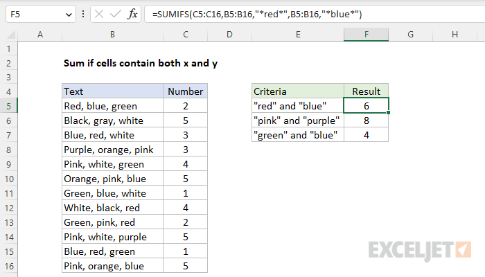
To sum numbers if cells contain both x and y (i.e., contain "red" and "blue") you can use the SUMIFS function. In the example shown, the formula in F5 is:
=SUMIFS(C5:C16,B5:B16,"*red*",B5:B16,"*blue*")
The result is 6, the sum of the numbers in column C when the text in column B contains both "red" and "blue" in any order. Note that SUMIFS is not case-sensitive.
Generic formula
=SUMIFS(sum_range,range,"*red*",range,"*blue*")
Explanation
In this example, the goal is to sum the numbers in column C when the text in column B contains specific pairs of colors. For example, the formula should sum a number when the text contains both "red" and "blue". Order is not important; the two colors can appear anywhere in the cell. However, both colors must appear in the same cell. This problem can be solved with the SUMIFS function, which is designed to sum numbers based on multiple criteria.
SUMIFS function
The SUMIFS function sums cells in a range that meet one or more conditions, referred to as criteria. The syntax for the SUMIFS function depends on the number of conditions needed. Each separate condition will require a range and criteria. The generic syntax for SUMIFS looks like this:
=SUMIFS(sum_range,range1,criteria1) // 1 condition
=SUMIFS(sum_range,range1,criteria1,range2,criteria2) // 2 conditions
In this case, we need two conditions, one to test for "red", and one to test for "blue". This means both criteria will be applied to the same range, the text in B5:B16. We start with the sum_range, which is the numbers in the range C5:C16:
=SUMIFS(C5:C16,
Then we add the first range/criteria pair to test for "red":
=SUMIFS(C5:C16,B5:B16,"*red*",
Note that we surround "red" with an asterisk () on either side. The asterisk () is a wildcard available in the SUMIFS function, which means "zero or more characters". We use a wildcard in this case to match "red" occurring anywhere in the text. Next, we add a second range/criteria pair to test for "blue" to complete the formula:
=SUMIFS(C5:C16,B5:B16,"*red*",B5:B16,"*blue*")
Again, we use two asterisks (*) as wildcards to match "blue" in any location. Notice we are applying two different criteria to the same range, B5:B15. This is intentional. The SUMIFS function applies criteria based on AND logic, which means that both conditions must be true for SUMIFS to include a value in the final result. In other words, both "red" and "blue" must exist in the text. Note that SUMIFS is not case-sensitive. Using "red" for criteria will match "Red", "RED", and "red" in any location.
Other combinations
The other color combinations in the worksheet shown use the same pattern. To test for "pink" and "purple", and "green" and "blue", the formulas in F6 and F7 are as follows:
=SUMIFS(C5:C16,B5:B16,"*pink*",B5:B16,"*purple*")
=SUMIFS(C5:C16,B5:B16,"*green*",B5:B16,"*blue*")