Summary
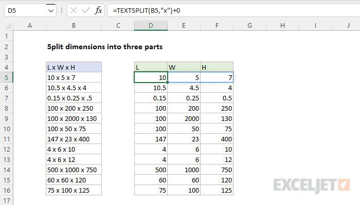
To split dimensions like "100x50x25" into three separate parts, you can use a formula based on the TEXTSPLIT function. In the example shown, the formula in cell D5 is:
=TEXTSPLIT(B5,"x")+0
The formula returns all three dimensions to cell D5, and the results spill into the range D5:F5.
Note: in older versions of Excel without TEXTSPLIT, you can use more complicated formulas based on several functions. Both approaches are explained below. Also, if you don't want or need to use a formula, you can use Excel's Text-to-Columns feature.
Generic formula
=TEXTSPLIT(A1,"x")+0
Explanation
In this example, the goal is to split the text strings in column B, which contain three dimensions in the form "L x W x H", into 3 separate dimensions. One problem with dimensions entered as text is that they can't be used for any kind of calculation. So, in addition, we want our final dimensions to be numeric. In a problem like this, we need to identify the delimiter, which is the character (or characters), that separate each thing we want to extract. In this case, the delimiter is the "x" character. Note that the "x" has a space (" ") on either side, something we'll also need to handle. Also notice that the "x" appears in different locations, so we can't extract dimensions by position.
There are two basic approaches to solving this problem. If you are using Excel 365, the easiest solution is to use the TEXTSPLIT function as shown in the worksheet above. If you are using an older version of Excel without TEXTSPLIT, you can use more complicated formulas based on several functions, including LEFT, RIGHT, LEN, SUBSTITUTE, and FIND. Both approaches are explained below.
TEXTSPLIT function
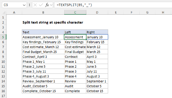
The TEXTSPLIT function is a great way to solve this problem, because it is so simple to use. To split dimensions into three parts, using the "x" as a delimiter, the formula in D5, copied down, is:
=TEXTSPLIT(B5,"x")+0
The formula works in two steps. First, TEXTSPLIT splits the text in B5 using the "x". The result is a horizontal array that contains three elements, one for each dimension:
={"10 "," 5 "," 7"}+0
Notice the numbers are still surrounded by space. Our goal is to get actual numeric values, so in the second step, we simply add zero. This is a simple way of getting Excel's formula engine to coerce a text value to an actual number. The result is an array like this:
={10,5,7} // true numbers
Notice the double quotes ("") are gone, because the math operation of addition (+) changes the text values to actual numbers. The formula returns this result to cell D5, and the three dimensions spill into the range D5:F5.
Note: one nice thing about the "add zero" trick, is that it doesn't matter if the number is surrounded by space characters or not. The numbers can be separated with " x " or "x" in the original text string with the same result. However, if you are splitting values that are not meant to be numbers, you will want to remove the +0, otherwise the formula will return a #VALUE! error.
Legacy Excel
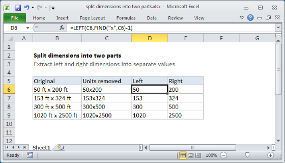
In Legacy Excel, we need to use more complicated formulas to accomplish the same thing. To get the first dimension (L), we can use a formula like this in D5:
=LEFT(B5,FIND("x",B5)-1)+0
At a high level, this works by extracting text starting from the left side. The number of characters to extract is calculated by locating the first "x" in the text using the FIND function, then subtracting 1:
=LEFT(B5,FIND("x",B5)-1)+0
=LEFT(B5,4-1)+0
=LEFT(B5,3)+0
="10 "+0
=10
To get the second dimension, we can use a formula like this in cell E5:
=MID(B5,FIND("x",B5)+1,FIND("~",SUBSTITUTE(B5,"x","~",2))-FIND("x",B5)-1)+0
At a high level, this formula extracts the width (W) with the MID function, which returns a given number of characters starting at a given position in the next. The starting position is calculated with the FIND function like this:
FIND("x",B5)+1
FIND simply locates the first "x" and returns the location (4) as a number. Then we add one to start at the first character after "x":
=FIND("x",B5)+1
=4+1
=5
The number of characters to extract, which is provided as num_chars to the MID function, is the most complicated part of the formula:
FIND("~",SUBSTITUTE(B5,"x","~",2))-FIND("x",B5)-1
Working from the inside out, we use SUBSTITUTE with FIND to locate the position of the 2nd "x", as described here. We then subtract from that the location of the first "x" + 1.
=FIND("~",SUBSTITUTE(B5,"x","~",2))-FIND("x",B5)-1
=FIND("~","10 x 5 ~ 7")-FIND("x",B5)-1
=8-FIND("x",B5)-1
=8-4-1
=3
The main trick here is that we are using the seldom seen instance_num argument in the SUBSTITUTE function to replace only the second instance of the "x" with a tilde (~), so that we can target the second instance of "x" with the FIND function in the next step.
Now that we've calculated the start_num and num_chars, we can simplify the original MID formula to this:
=MID(B5,5,3)+0
=MID("10 x 5 x 7",5,3)+0
=" 5 "+0
=5
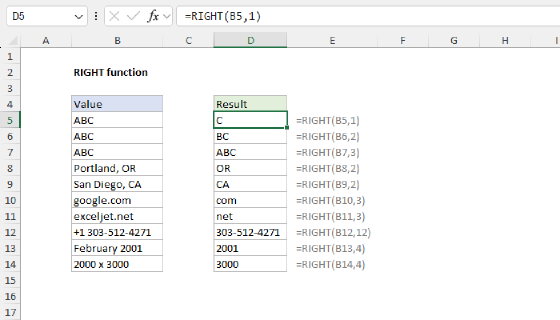
Note we are using the trick of adding zero again to force Excel to coerce the next to a number. Finally, to get the third dimension, we can use a formula like this in cell F5:
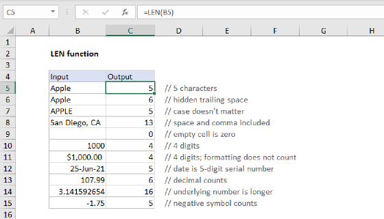
=RIGHT(B5,LEN(B5)-FIND("~",SUBSTITUTE(B5,"x","~",2)))+0
This formula works a lot like the formula to get the second dimension above. At a high level, we are using the RIGHT function to extract text from the right. The main challenge is to calculate how many characters to extract, num_chars, which is done again with FIND and SUBSTITUTE like this:
LEN(B5)-FIND("~",SUBSTITUTE(B5,"x","~",2))
As above, we use 2 for instance_num argument in the SUBSTITUTE function to replace only the second instance of the "x" with a tilde (~), so that we can target this instance of "x" with the FIND function in the next step:
=LEN(B5)-FIND("~",SUBSTITUTE(B5,"x","~",2))
=RIGHT(B5,10-8)+0
=RIGHT(B5,2)+0
=" 7"+0
=7
The LEN function returns the total characters in the text string (10) and FIND returns 8 as the location of the second "x", so num_chars becomes 2 in the end. RIGHT returns the 2 characters from the right side of the text string (which includes a space) we add zero to the result to force Excel to change the next to a number.