Summary
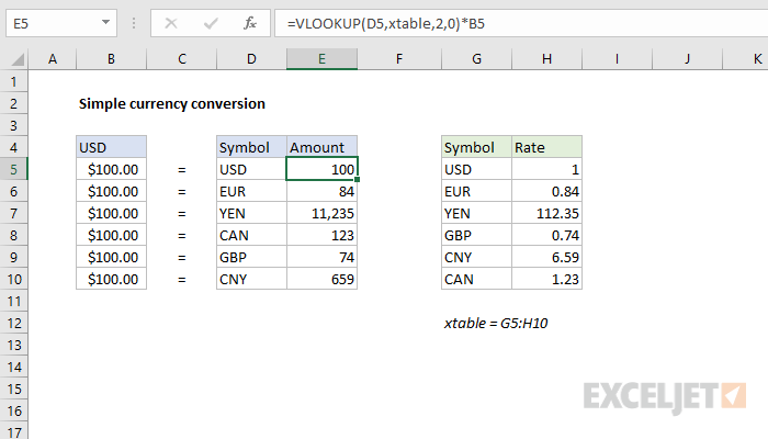
To convert from a given currency to other specific currencies, you can use the VLOOKUP function with a lookup table that contains conversion rates. In the example shown, the formula in E5 is:
=VLOOKUP(D5,xtable,2,0)*B5
Where "xtable" is the named range G5:H10. As the formula is copied down, it converts the amount in column B from US Dollars (USD) to the currency indicated in column D.
Generic formula
=VLOOKUP(currency,xtable,column,0)*amount
Explanation
The formula in this example converts amounts in USD to other currencies using currency codes and a simple lookup table. The available currencies and exact conversion rates can be adjusted by editing the values in the table on the right. The core of this formula is the VLOOKUP function, configured like this:
=VLOOKUP(D5,xtable,2,0)
The inputs to VLOOKUP are given as follows:
- lookup_value - the currency code in D5
- table_array - the currency conversion table in G5:H10, given as the named range xtable
- col_index_num - 2, because we want to return values from column H
- range_lookup - 0, because we want VLOOKUP to perform an exact match
For more information on VLOOKUP, see this detailed overview.
In this configuration, VLOOKUP finds the currency in the table and retrieves the conversion rate from column H. The result from VLOOKUP is then multiplied by the value in B5, which is the number of US dollars to convert.
Note: If a currency code does not exist in the table, VLOOKUP will return a #N/A error.
Nested IF equivalent
Note that it is possible to build a formula to do a currency conversion by nesting multiple IF functions together and hardcoding the currency rates directly into the formula like this:
=IF(D5="usd",1,
IF(D5="eur",0.84,
IF(D5="yen",112.35,
IF(D5="can",1.23,
IF(D5="gpb",0.74,
IF(D5="cny",6.59))))))*B5
Note: in the formula above, line breaks have been added for better readability.
I present this option here to illustrate how the VLOOKUP option is superior. It's a much simpler formula, and the exchange rate values are not stored redundantly in many different formulas. In addition, keeping the lookup table on the worksheet makes it easy to see and edit the exchange rates (in one place) at any time.