Summary
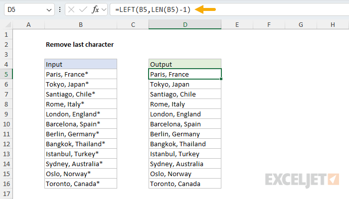
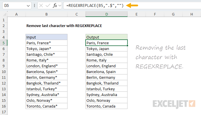
To remove the last character(s) from a text string, you can use a formula based on the LEFT and LEN functions. In the worksheet shown above, each city and country in column B ends with an asterisk (*) that we would like to remove. We do it with a formula like this in cell D5:
=LEFT(B5,LEN(B5)-1)
As the formula is copied down, it uses the LEFT function to remove the last character in each text string. The values in column D show the result.
This formula will work in all versions of Excel. The article below also explains a fancy new way to do the same thing with the REGEXREPLACE function, which requires the latest version of Excel.
Generic formula
=LEFT(text,LEN(text)-n)
Explanation
In this example, the goal is to remove the asterisk (*) at the end of each text city/country name in column B. As usual, there are many ways to solve a problem like this in Excel. In the article below, we'll look at two good options. The first is a traditional formula based on the LEFT function and the LEN function. This formula will work in any version of Excel. The second option is a formula based on the REGEXREPLACE function, which was recently introduced to Excel. The REGEXREPLACE approach is more powerful and flexible, but it is only available in the latest version of Excel.
If you only want to remove trailing spaces from a text string, the TRIM function is faster and easier. In one step, it can remove leading and trailing spaces and normalize the space between words.
Table of Contents
- Remove the last character
- Remove the last 3 characters
- REPLACE function alternative
- Remove the last character with REGEXREPLACE
- Remove the last 3 characters with REGEXREPLACE
- Making the formulas conditional
Note, the formulas on this page are configured to remove asterisks (*) because they are easy to see and understand. However, these formulas can be adapted to remove specific characters or a specific number of characters, as explained below. I realize you could use the SUBSTITUTE function to remove specific text anywhere in a text string. 🙂
Remove the last character
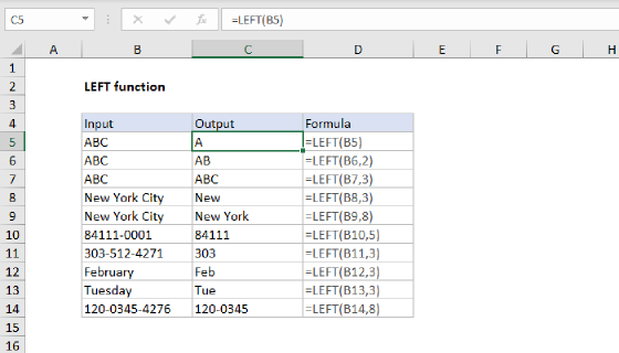
The traditional way to solve this problem in Excel is to combine the LEFT and LEN functions. The LEFT function returns characters starting at the left side of a text string:
=LEFT("apple",3) // returns "app"
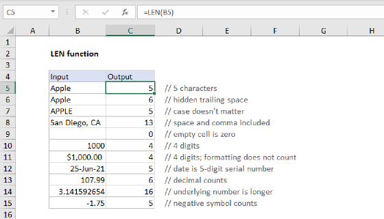
The LEN function returns the length of a text string:
=LEN("apple") // returns 5
To solve this problem, we want to get all of the characters starting at the left and ending at the character before the asterisk (*) at the end. To do this, we can nest the LEN function inside the LEFT function to return the length of the string and then subtract one to remove the last character, like this:
=LEFT(B5,LEN(B5)-1)

This is how the formula works:
=LEFT(B5,LEN(B5)-1)
=LEFT(B5,14-1)
=LEFT(B5,13)
="Paris, France"
- The LEN function returns 14 because "Paris, France*" contains 14 characters.
- We subtract 1, and the result (13) is passed to LEFT as num_chars.
- The LEFT function returns the first 13 characters of the text, skipping the last character.
- The final result is "Paris, France", without the asterisk.
- As the formula is copied down, the process repeats for each city in the list.
Remove the last 3 characters
What if you want to remove more than one character from the end of a text string? The general form of the formula looks like this, where n represents the number of characters to remove:
=LEFT(A1,LEN(A1)-n)
This means we just need to change n to the number of characters we'd like to remove. For example, in the worksheet below, we have the same city and country names, but now each one is followed by three asterisks. The formula in cell D5 now looks like this:
=LEFT(B5,LEN(B5)-3)
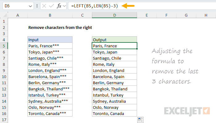
The formula works the same way as the example above, but now, because we are subtracting 3 from the length of the text string, the result is that we removed the last three characters from the right side. It's always a little confusing that we use the LEFT function to remove characters from the right side of the text string, but that's just the way this works 🙃.
REPLACE function alternative
Although the formula based on the LEFT and LEN functions works fine, I should mention that you can write a similar formula based on the REPLACE function. The generic formula to remove the last n characters looks like this:
=REPLACE(A1,LEN(A1)-n+1,n,"")
This formula will replace n characters in A1 with an empty string (""), starting at the position calculated with LEN(A1)-n+1. Both options are solid and will work in any version of Excel.
Remove the last character with REGEXREPLACE
The formula based on LEFT and LEN explained above is a traditional formula that will work in all versions of Excel. If you have the latest version of Excel, which includes three new regex functions, you have a more powerful tool at your disposal. In the worksheet below, I have converted the formula to use the REGEXREPLACE function to remove the last character. The formula in D5 now looks like this:
=REGEXREPLACE(B5,".$","")
Notice that we only have a single function call for this solution. The inputs to REGEXREPLACE are as follows:
- text -
B5 - pattern -
".$" - replacement -
""
At a high level, we are replacing the last character in B5 with an empty string (""). The trick is in how we match the last character, which is done with the pattern ".$". In regex, a single dot (.) will match any character. The dollar sign ($) is a special anchor character that matches the end of a text string. The result is a pattern that matches the last character at the end of the text string. See a related example here.
Remove the last 3 characters with REGEXREPLACE
How do we use regex to target the last three characters? This is an example that shows off the flexibility of regex patterns. Regex has something called quantifiers that you can use to specify how many instances of a character you want to match. In this case, we can use a form like {n} to specify n characters, so {3} to match 3 characters. You can see this in the worksheet below, where the formula in D5 now looks like this:
=REGEXREPLACE(B5,".{3}$","")
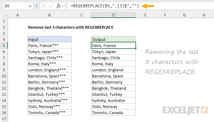
As before, we are using REGEXREPLACE to replace text that matches a specific pattern with an empty string. The pattern in this case is ".{3}$", which breaks down as follows:
- The
.matches any single character. - The
{3}means “exactly three”. - The
$anchors the match to the end of the string.
Making the formulas conditional
In this kind of problem, one challenge that comes up often is that you only want to remove certain characters at the end of a text string if they exist. Otherwise, you might chop off characters you want to keep. In other words, we want to make the formulas conditional. Let's look at how to do that with both the traditional LEFT + LEN formula and the newer formula based on regex replace. For the first formula, I think the simplest way to do this is to test the string directly with the IF function and the RIGHT function like this:
=IF(RIGHT(B5,1)="*",LEFT(B5,LEN(B5)-1),B5)
Here we use the RIGHT function to extract the last character and check if it is an asterisk (). If so, we run the original formula that removes the last character. If not, we would return the original value unchanged. To make the regex replace formula conditional, we could use the IF function as above to check for the asterisk () in the same way:
=IF(RIGHT(B5,1)="*",REGEXREPLACE(B5,".$",""),B5)
However, a simpler option is to adjust the pattern to match a literal asterisk (*) at the end of the text:
=REGEXREPLACE(B5,"\*$","")
The pattern "\*$" works like this:
- The
\*matches a literal asterisk (*) - The
$anchors the match to the end of the string.
What's the backslash \ doing in there? There are certain characters in regex (like *) that need to be escaped. This is because these characters have other meanings. For example, the asterisk (*) by itself means "match zero or more times" when it appears as a quantifier in a pattern. The backslash is a way to specify these characters literally. So, "\*$" matches a literal asterisk that appears at the end of a text string. This means the match will fail if the * is not at the end of a text string, or if it appears anywhere else in the text. And, if the match fails, REGEXREPLACE returns the original value unchanged.
Tip: Escape other regex metacharacters the same way, for example
\+$for a trailing plus sign.
In the worksheet below, notice that only some cities in column B are followed by an asterisk (*). To avoid removing characters from cities that do not have an asterisk, we need conditional formulas. In cell D5, we use the traditional formula wrapped in IF to check for the asterisk before processing:
=IF(RIGHT(B5,1)="*",LEFT(B5,LEN(B5)-1),B5)
In cell F5, we have the REGEXREPLACE alternative:
=REGEXREPLACE(B5,"\*$","")
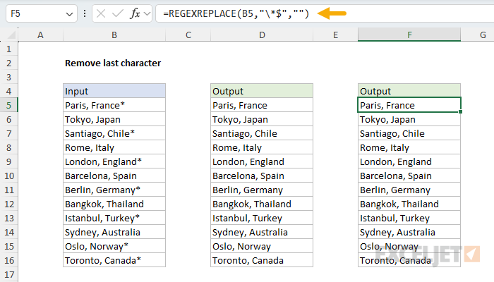
You can see that both formulas correctly remove the last character from cities that end in an asterisk. Cities that do not end in an asterisk are returned unchanged.
I should also mention that you could use the pattern
\*+$to remove any number of trailing asterisks. Regex has a huge number of special symbols that can be adapted in many ways for very specific matching. See our quick reference table for examples.
I think this is a good example of how regex patterns are a much more powerful way to target specific text. In the traditional formula, the LEFT and LEN functions have no idea what they're doing. They're simply chopping off characters. Any control over which characters are being removed needs to be added to the formula in the form of other functions. By contrast, the REGEXREPLACE function can use regular expressions to target specific text precisely, with built-in tools to make the match conditional. The trade-off is that Excel's regex functions require at least some familiarity with regular expressions.