Summary
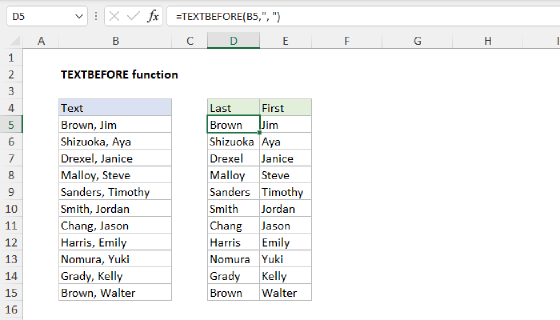
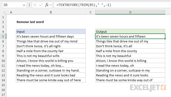
To remove the last word from a text string, you can use a formula based on the TEXTBEFORE function together with the TRIM function. In the example shown, the formula in cell D5, copied down, is:
=TEXTBEFORE(TRIM(B5)," ",-1)
As the formula is copied down, it removes the last word from each text string in column B.
Note: TEXTBEFORE is only available in newer versions of Excel. See below for a formula that will work in older versions.
Generic formula
=TEXTBEFORE(TRIM(B5)," ",-n)
Explanation
In this example, the goal is to remove the last word from the text strings in column B. This article explains two approaches:
- A modern formula based on the TEXTBEFORE function.
- A more traditional formula for older versions in Excel.
The first option is much simpler, and you should use it if you have the TEXTBEFORE function. The second formula is significantly more complex and only makes sense if you don't have TEXTBEFORE.
This formula is a great example of how new functions in Excel completely change how problems are solved. The traditional formula is much more complex than the modern formula.
Modern formula based on TEXTBEFORE
In the latest version of Excel, we can easily solve this problem with the TEXTBEFORE function. TEXTBEFORE is designed to extract text that occurs before a given delimiter with a syntax like this:
=TEXTBEFORE(text,delimiter)
For example, we can extract "Bob" from "Bob Alan Jones" by using a space as a delimiter like this:
=TEXTBEFORE("Bob Alan Jones"," ") // returns "Bob"
The third argument for TEXTBEFORE is called "instance_num" and specifies the instance of the delimiter as a numeric index (i.e., instance 1, instance 2, instance 3, etc.) This argument is optional and defaults to 1. This is why we get "Bob" when we don't provide a value for instance_num. If we set instance_num to 2, we get "Bob Alan":
=TEXTBEFORE("Bob Alan Jones"," ",2) // returns "Bob Alan"
The instance number can also be provided as a negative number, which counts from the end of the text string:
=TEXTBEFORE("Bob Alan Jones"," ",-2) // returns "Bob"
=TEXTBEFORE("Bob Alan Jones"," ",-1) // returns "Bob Alan"
This feature is the key to using TEXTBEFORE to solve this problem. Since we don't know how many words a text string will contain, we don't know what (positive) instance number to provide to TEXTBEFORE to target text before the last word. However, if we switch to a negative instance number, we can easily target the last word by using -1 for instance_num. The meaning is "first space from the end" which is the same as "last space from the start". The formula looks like this:
=TEXTBEFORE(B5," ",-1)
This will work fine as long as the text string in B5 always contains words separated by just one space (" "). However, if the number of spaces between words is irregular, or if there are extra spaces after the text, the formula may not work correctly. To avoid this problem, we ensure the spacing is consistent by nesting the TRIM function inside TEXTBEFORE:
=TEXTBEFORE(TRIM(B5)," ",-1)
Inside TEXTBEFORE, the TRIM function normalizes the space in the text string from cell B5. TRIM makes sure there is just one space between words and removes any leading or trailing spaces. The "trimmed" text is returned directly to TEXTBEFORE as the text argument. The TEXTBEFORE function then returns all text before the last word, effectively removing the last word.
Customizing the modern formula
Since this formula is so simple, it's easy to customize its behavior. To remove more than the last word (i.e., the last two words, the last three words, etc.), we only need to adjust the instance number:
=TEXTBEFORE(TRIM(A1)," ",-1) // remove last word
=TEXTBEFORE(TRIM(A1)," ",-2) // remove last two words
=TEXTBEFORE(TRIM(A1)," ",-3) // remove last three words
The generic formula to return the last n words looks like this:
=TEXTBEFORE(TRIM(A1)," ",-n)
Note: If you provide a value for n that is out of range, TEXTBEFORE will return a #N/A error.
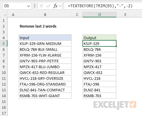
We can also easily change the delimiter used to separate words. For example, to remove the last 2 words separated by hyphens, we can use a formula like this:
=TEXTBEFORE(TRIM(A1),"-",-2)
You can see how this works in the worksheet below:
Traditional formula for older versions of Excel
In older versions of Excel, this is a much harder problem to solve because there is no easy way to split text at the last space. A classic traditional formula solution looks like this:
=MID(B5,1,FIND("~",SUBSTITUTE(B5," ","~",LEN(B5)-LEN(SUBSTITUTE(B5," ",""))))-1)
At the highest level, this formula uses the MID function to remove the last word from a text string. The challenge is to figure out where the last word begins and set a marker before the last word. Then, we can locate the marker with FIND and extract everything up to that point. The formula is convoluted, but the steps are simple. First, we count how many spaces exist in the text using LEN and SUBSTITUTE like this:
LEN(B5)-LEN(SUBSTITUTE(B5," ","")) // returns 6
This page explains this part of the formula in more detail. Next, we use the somewhat obscure instance argument in the SUBSTITUTE function to replace the last space with a tilde (~):
SUBSTITUTE(B5," ","~",6) // insert tilde
We use a tilde (~) only because it's a rarely occurring character. You can use any character you like, so long as it doesn't appear in the source text.
At this point in the process, the formula looks like this:
=MID(B5,1,FIND("~","It's been seven hours and fifteen~days")-1)
Notice that the tilde (~) acts as a marker to indicate where the last word begins. Next, we use FIND to figure out where the tilde is:
FIND("~","It's been seven hours and fifteen~days") // returns 34
FIND returns 34 because the tilde is the 34th character in the text string. Because we don't want to extract the tilde itself, we subtract 1 from the number that FIND returns. The result, 33, is returned to the MID function as the num_chars argument. We are finally ready to extract text. At this point, we can simply the formula as follows:
=MID(B5,1,33)
The MID function extracts all text from character 1 through character 33, effectively removing the last word from the original text in cell B5.
This formula is a great example of how new functions in Excel completely change how tricky problems are solved. The traditional formula is much more complex and much less transparent than the TEXTBEFORE solution. Plus, we haven't even accounted for irregular spacing, which would require adding the TRIM function around each instance of B5 in the formula, which would make the formula even more complicated.
Customizing the traditional formula
The same formula structure can be used with a different delimiter. For example, to remove all text after the last forward slash "/", you can use a generic formula like this:
=MID(A1,1,FIND("~",SUBSTITUTE(A1,"/","~",LEN(A1)-LEN(SUBSTITUTE(A1,"/",""))))-1)
You can also adapt the formula to remove the last 2 words, last 3 words, etc. The general form for this formula looks like this:
=MID(A1,1,FIND("~",SUBSTITUTE(A1,d,"~",LEN(A1)-LEN(SUBSTITUTE(A1,d,""))-(n-1)))-1)
In the above formula, n is the number of words to remove, and d represents the delimiter to use.