Random numbers without duplicates

In this example, the goal is to generate a list of random numbers without duplicates. This involves jumping through a few hoops because although the RANDARRAY function can easily generate a list of random integers, there is no guarantee that the numbers will be unique. In the explanation below, we'll look first at a simple option with the RANDARRAY function, then at a more complete solution based on the SEQUENCE function.

Background study

• New dynamic array functions in Excel - 3 min video
• How to perform a random sort - 3 min video

RANDARRAY option

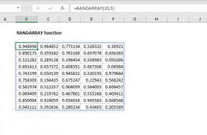
The RANDARRAY function makes it easy to generate a list of random integers. For example, to generate 12 random numbers between 1 and 100, you can use RANDARRAY like this:

=RANDARRAY(12,1,1,100,TRUE)

The rows argument sets how many numbers are returned, columns is 1, start is 1, end is 100, and integer is set to TRUE. This formula works fine. However, if you enter the formula and press F9 a few times, you will likely see some duplicate numbers because there is no guarantee that the numbers are unique.

By increasing the range of numbers generated, we can reduce the possibility of duplicates substantially. For example, this formula returns 12 random numbers between 10000 and 50000:

=RANDARRAY(12,1,10000,50000,TRUE)

Although there is still a possibility of duplicates, the chance is much lower since there are 40,002 possible numbers. To ensure that there are no duplicates, we can wrap RANDARRAY inside the UNIQUE function like this:

=UNIQUE(RANDARRAY(12,1,10000,50000,TRUE))

The formula above works well if a specific number of results is not required. However, because the UNIQUE function will remove duplicates if they exist, the final count of numbers returned will change. To work around this problem, and ensure a fixed number of unique random numbers, we can take a different approach with the SEQUENCE function as described below.

Random sort

Another approach is to use the SEQUENCE function to generate a unique list of numbers, then use SORTBY and RANDARRAY to sort the list randomly. For example, to return 15 numbers sorted randomly, you can use a formula like this:

=SORTBY(SEQUENCE(15),RANDARRAY(15))

SEQUENCE returns an array of numbers between 1-15, RANDARRAY returns an array of 15 decimal values, and the SORTBY function sorts the output from SEQUENCE using the output from RANDARRAY. The result is a list of the 15 numbers between 1-15, sorted randomly.

Random sort and extract

An alternative to the simple approach described above is to create a list of unique numbers with the SEQUENCE function, sort the list randomly, and then extract a portion of the list. This guarantees a specific number of unique values across a large range of possibilities. This is the approach used in the worksheet shown above, where the formula in cell F5 is:

=INDEX(SORTBY(SEQUENCE(C5,1,C4,C6),RANDARRAY(C5)),SEQUENCE(C7))

Replacing the cell references with their values, we have:

=INDEX(SORTBY(SEQUENCE(1000,1,10000,10),RANDARRAY(1000)),SEQUENCE(12))

Working from the inside out, the core of the formula is this:

SORTBY(SEQUENCE(1000,1,10000,10),RANDARRAY(1000))

At a high level, the SORTBY function is used to sort the output from SEQUENCE randomly. The SEQUENCE function is configured to generate 1000 numbers starting at 10000. The step argument is given as 10 to return numbers that are multiples of 10. The result from SEQUENCE is an array that contains 1000 numbers. The first 10 numbers in the array look like this:

{10000;10010;10020;10030;10040;10050;10060;10070;10080;10090;...}

These numbers are returned directly to SORTBY as the array argument.

The RANDARRAY function is set to output 1000 numbers. By default, RANDARRAY will return an array of long decimals. The first 10 numbers in the array will look something like this:

{0.568145559543193;0.0442765690172342;0.682220112357301;0.293859840996845;0.0875380500249507;0.0872080540305316;0.384740824003848;0.8250435788655;0.698609517138334;0.844906019655289;...}

These numbers are provided to SORTBY as the by_array1 argument. With the result from SEQUENCE as array, and the result from RANDARRAY as by_array1, SORTBY sorts all 1000 numbers randomly and returns the sorted array to the INDEX function. If we refer to this randomly sorted array  as "random_array", we can simplify and rewrite the original formula like this:

=INDEX(random_array,SEQUENCE(C7))

Here, random_array is delivered to INDEX as the array argument. The SEQUENCE function creates an array with the numbers 1-12, and returns this array to INDEX as the row_num argument:

=INDEX(random_array,{1;2;3;4;5;6;7;8;9;10;11;12})

With these inputs, INDEX returns the first 12 rows from the randomly sorted array as a final result. The numbers are guaranteed to be unique because the original array created by SEQUENCE contains no duplicates.

Random names

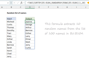
The approach described above can be applied to other related problems. For example, once you have a list of random numbers without duplicates, you can use those numbers with the INDEX function to create a random list of names without duplicates.

Legacy Excel

Dynamic array formulas are a new feature in Excel. If you have a version of Excel without SEQUENCE, SORTBY, and RANDARRAY, you can take a more manual approach. One method is to enter the core set of numbers to choose from in one column, and use the RAND function to assign random decimal values to each number in another column. Then you can use an INDEX and MATCH formula with the LARGE function to extract random numbers according to their numeric rank. The screen below shows the basic idea:

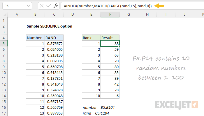
The formula in F5, copied down, is:

=INDEX(number,MATCH(LARGE(rand,E5),rand,0))

where number (B5:B104) and rand (C5:C104) are named ranges. The LARGE function is used to get the nth largest random decimal number in C5:C104, where n comes from column E. LARGE returns this value to the MATCH function as lookup_value, which locates the position of the value in the random decimal values. MATCH returns this position to the INDEX function, and INDEX returns the number at that position in B5:B104. The final result is 10 random numbers between 1-100 in F5:F14 without duplicates.