Excel formula: List most frequently occuring numbers

Generic formula

{=MODE(IF(1-ISNUMBER(MATCH(data,exp_rng,0)),data))}

Summary

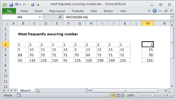
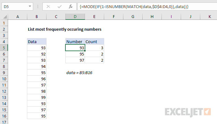
To list the most frequently occurring numbers in a column (i.e. most common, second most common, third most common, etc), you can an array formula based on four Excel functions, IF, MODE, MATCH, and ISNUMBER. In the example shown, the formula in D5 is:

{=MODE(IF(1-ISNUMBER(MATCH(data,$D$4:D4,0)),data))}

where "data" is the named range B5:B16. The formula is then copied to rows below D5 to output the desired list of most frequent numbers.

Note: this is an array formula and must be entered with control + shift + enter.

Explanation

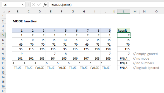
The core of this formula is the MODE function, which returns the most frequently occurring number in a range or array. The rest of the formula just constructs a filtered array for MODE to use in each row. The expanding range $D$4:D4 works to exclude numbers already output in $D$4:D4.

Working from the inside out:

MATCH function is used first check all numbers in the named range "data" against existing numbers in the expanding range $D$4:D4
ISNUMBER converts matched values to TRUE and non-matched values to FALSE
1-NUMBER reverses the array, and the math operation outputs ones and zeros
IF uses the array output of #3 above to filter the original list of values, excluding numbers already in $D$4:D4
The MODE function returns the most frequent number in the array output in step #4

In cell D5, no filtering occurs and the output of each step above looks like this:

{#N/A;#N/A;#N/A;#N/A;#N/A;#N/A;#N/A;#N/A;#N/A;#N/A;#N/A;#N/A}
{FALSE;FALSE;FALSE;FALSE;FALSE;FALSE;FALSE;FALSE;FALSE;FALSE;FALSE;FALSE}
{1;1;1;1;1;1;1;1;1;1;1;1}
{93;92;93;94;95;96;97;98;99;93;97;95}
93

In cell D6, with 93 already in D5, the output looks like this:

{2;#N/A;2;#N/A;#N/A;#N/A;#N/A;#N/A;#N/A;2;#N/A;#N/A}
{TRUE;FALSE;TRUE;FALSE;FALSE;FALSE;FALSE;FALSE;FALSE;TRUE;FALSE;FALSE}
{0;1;0;1;1;1;1;1;1;0;1;1}
{FALSE;92;FALSE;94;95;96;97;98;99;FALSE;97;95}
95

Handling errors

The MODE function will return the #N/A error when there is no mode. As you copy the formula down into subsequent rows, you will likely run into the #N/A error. To trap this error and return an empty string instead, you can use IFERROR like this:

=IFERROR(MODE(IF(1-ISNUMBER(MATCH(data,$D$4:D4,0)),data)),"")

Author

Dave Bruns

Related formulas

Most frequently occurring text

Working from the inside out, the MATCH function matches the range against itself. That is, we give the MATCH function the same range for lookup value and lookup array (B5:F5). Because the lookup value contains more than one value (an array), MATCH...

Most frequently occurring number

The MODE function is fully automatic and will return the most frequently occurring number in a set of numbers. For example: = MODE ( 1 , 2 , 4 , 4 , 5 , 5 , 5 , 6 ) // returns 5 In the example shown, we give MODE the range B4:K4, so the formula is...

Filter values in array formula

The MATCH function checks all values in the named range "data" against values in "filter" ISNUMBER converts matched values to TRUE and non-matched values to FALSE IF uses the array output in #2 above to filter values, excluding values in "filter"...

Related functions

Excel MODE Function

The Excel MODE function returns the most frequently occurring number in a numeric data set. For example, =MODE(1,2,4,4,5,5,5,6) returns 5.

Excel ISNUMBER Function

The Excel ISNUMBER function returns TRUE when a cell contains a number, and FALSE if not. You can use ISNUMBER to check that a cell contains a numeric value, or that the result of another function is a number.

Excel MATCH Function

MATCH is an Excel function used to locate the position of a lookup value in a row, column, or table. MATCH supports approximate and exact matching, and wildcards (* ?) for partial matches. Often, MATCH is combined...

Excel Formula Training

Formulas are the key to getting things done in Excel. In this accelerated training, you'll learn how to use formulas to manipulate text, work with dates and times, lookup values with VLOOKUP and INDEX & MATCH, count and sum with criteria, dynamically rank values, and create dynamic ranges. You'll also learn how to troubleshoot, trace errors, and fix problems. Instant access. See details here.