Summary
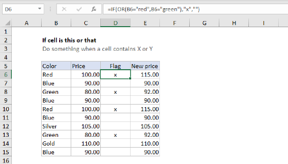
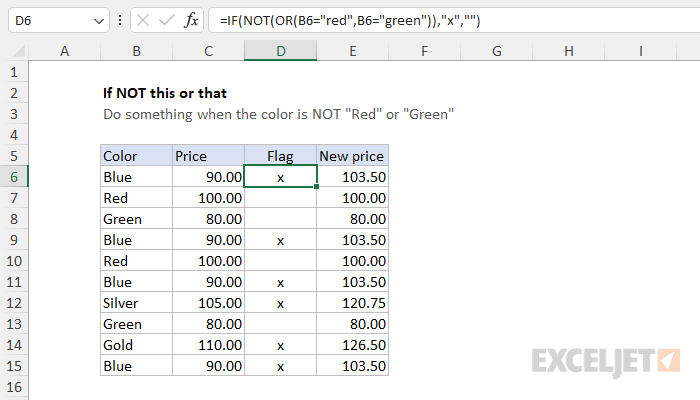
To do something when a cell is NOT this or that (i.e. a cell is NOT equal to "x", "y", etc.) you can use the IF function together with the OR function and the NOT function. In cell D6, the formula is:
=IF(NOT(OR(B6="red",B6="green")),"x","")
When copied down, it returns "x" when the color in column B contains any value except "red" or "green". Otherwise, the formula returns an empty string ("") which looks like an empty cell in Excel. Notice that Excel is not case-sensitive by default, B6="red", B6="Red", and B6="RED" will all return the same result.
Generic formula
=IF(NOT(OR(A1="red",A1="green")),"x","")
Explanation
The goal is to "flag" records that are neither "Red" nor "Green". More specifically, we want to check the color in column B, and leave an "x" in rows where the color is NOT "Red" OR "Green". If the color is "Red" OR "Green", we want to display nothing.
IF function logic
The IF function is commonly used for simple tests. For example, to return "OK", when a value is over 100 and "Fail" if not, you can use the IF function in a formula like this:
=IF(A1>100,"OK","Fail")
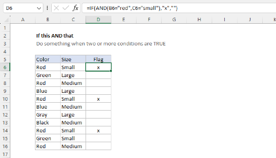
In this formula, A1>100 is the logical test. The behavior of the IF function can be easily extended by adding functions like AND, OR, and NOT to the logical test. For example, to reverse the existing logic in the formula above, we can add NOT like this:
=IF(NOT(A1>100),"OK","Fail")
Translation: If the value in A1 is NOT greater than 100, then return "OK". Otherwise, return "Fail".
In the worksheet shown, the goal is to mark records where the color is NOT "Red" OR "Green" with an "x". If the color is "Red" or "Green" we don't want to do anything. The formula in cell D6 is:
=IF(NOT(OR(B6="red",B6="green")),"x","")
In this formula, the logical test is this bit:
NOT(OR(B6="red",B6="green"))
Working from the inside out, we first use the OR function to test for "red" or "green":
OR(B6="red",B6="green")
OR will return TRUE if B6 is "Red" or "Green", and FALSE if B6 contains any other value. The NOT function simply reverses this result. Adding NOT means the test will return TRUE if B6 is NOT "Red" or "Green", and FALSE otherwise:
NOT(OR(B6="red",B6="green"))
The rest of the formula is standard. Since we want to flag items that pass the test, we provide "x" for value_if_true. Since we don't want to display anything for other values, we provide an empty string ("") for value_if_false. This causes an "x" to appear in column D when the color in column B is NOT "Red" or "Green". You can extend the OR function to check additional conditions as needed.
Keep in mind that Excel is not case-sensitive by default, so the color names in the formula are all lowercase. The expressions B6="red", B6="Red", and B6="RED" will all return the same result. Also, notice that we need to provide an empty string ("") for the false result. This argument is not required, but if we leave it empty, the formula will return FALSE when a color is "Red" or "Green".
Increase price
You can use other formulas inside the IF function to run a different calculation instead of simply returning "x". For example, let's say you want to increase the price for all colors except Red and Green by 15%. If the color is Red or Green, you want to leave the price alone. To perform this task, the formula in E6 below is:
=IF(NOT(OR(B6="red",B6="green")),C6*1.15,C6)
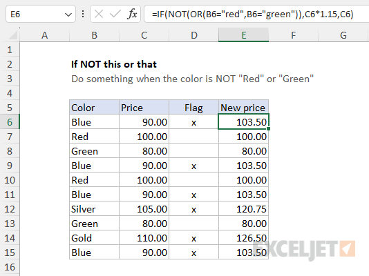
Translation: if the color is NOT "Red" or "Green", increase the price by 15%. Otherwise, return the original price.