If not blank multiple cells

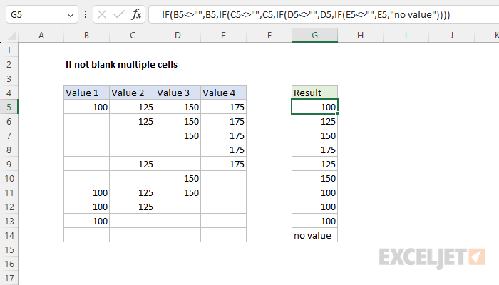
To test multiple cells, and return the value from the first non-blank cell, you can use a formula based on the IF function. In the example shown, the formula in cell G5 is:

=IF(B5<>"",B5,IF(C5<>"",C5,IF(D5<>"",D5,IF(E5<>"",E5,"no value"))))

The result is the first non-blank cell: B5, C5, D5, or E5, respectively. When all cells are blank, the formula returns "no value". The value returned when all cells are blank can be adjusted as desired.

Feeling underwhelmed by the manual complexity of this formula? See below for a more elegant solution based on the XLOOKUP function. -Dave

Explanation

The goal is to return the first non-blank value in each row from columns B:E, moving left to right. One way to solve this problem is with a series of nested IF statements. Since all cells are contiguous (connected) another way to get the first value is with the XLOOKUP function. Both approaches are explained below.

Nested IF solution

In the worksheet shown, the formula in cell G5 is:

=IF(B5<>"",B5,IF(C5<>"",C5,IF(D5<>"",D5,IF(E5<>"",E5,"no value"))))

In Excel, empty double quotes ("") mean an empty string. The <> symbol is a logical operator that means "not equal to", so the following expression means "A1 is not empty":

=B5<>"" // B5 is not empty

The overall structure of this formula is what is called a "nested IF formula". Each IF statement checks a cell to see if a particular cell is not empty. If a cell is not empty, the IF returns the value from that cell. If the cell is empty, the IF statement hands off processing to the following IF function. The flow of a nested IF is somewhat easier to understand if we add line breaks to the formula to separate each IF function like this:

=
IF(B5<>"",B5,
IF(C5<>"",C5,
IF(D5<>"",D5,
IF(E5<>"",E5,
"no value"))))

Video: How to make a nested if formula easier to read

With ISBLANK

It is also possible to use the ISBLANK function, which returns TRUE when a cell is blank:

=ISBLANK(A1) // A1 is blank

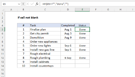
The behavior can be "reversed" by nesting the ISBLANK function inside the NOT function:

=NOT(ISBLANK(A1)) // A1 is not blank

The original formula above can be re-written to use ISBLANK as follows:

=IF(NOT(ISBLANK(B5)),B5,IF(NOT(ISBLANK(C5)),C5,IF(NOT(ISBLANK(D5)),D5,IF(NOT(ISBLANK(E5)),E5,"novalue"))))

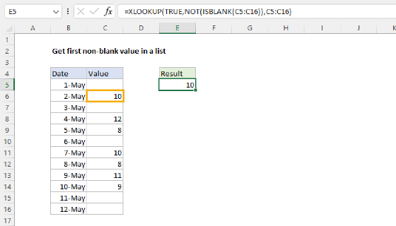
XLOOKUP solution

Another way to solve this problem is with the XLOOKUP formula like this:

=XLOOKUP(TRUE,ISNUMBER(B5:E5),B5:E5)

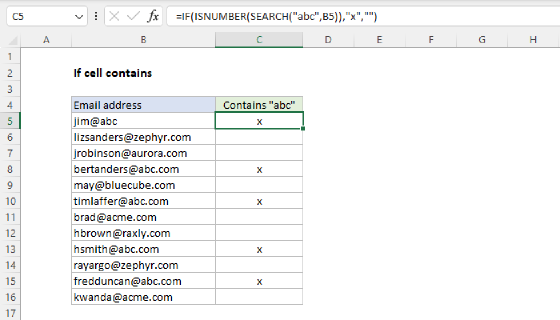
We can use XLOOKUP in this case because the four cells in B5:E5 are together, so can be provided as a single range. The ISNUMBER function checks the range and returns an array of TRUE and FALSE values like this:

{TRUE,TRUE,TRUE,TRUE}

XLOOKUP matches the first TRUE in the array and returns the corresponding value in B5:E5. Note that this approach only works because all the cells being checked are in a contiguous range. You can read more about XLOOKUP here.