If cell contains one of many things

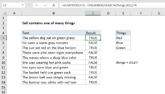
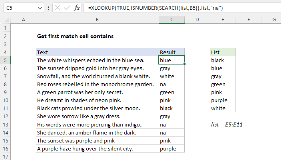
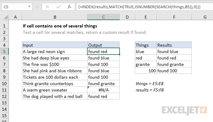
To test a cell for one of several strings, and return a custom result for the first match found, you can use an INDEX / MATCH formula based on the SEARCH function. In the example shown, the formula in C5 is:

{=INDEX(results,MATCH(TRUE,ISNUMBER(SEARCH(things,B5)),0))}

where things (E5:E8 ) and results (F5:F8) are named ranges. This is an array formula and must be entered with Control + Shift + Enter.

Note: this formula is designed to return a different result for each value that may be found. If you only want to test for one of many values and return a single result when found, see this formula.

Explanation

This formula uses two named ranges: things, and results. If you are porting this formula directly, be sure to use named ranges with the same names (defined based on your data). If you don't want to use named ranges, use absolute references instead.

The core of this formula is this snippet:

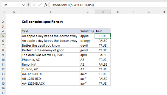
ISNUMBER(SEARCH(things,B5)

This is based on another formula (explained in detail here) that checks a cell for a single substring. If the cell contains the substring, the formula returns TRUE. If not, the formula returns FALSE.

Because we are giving the SEARCH function more than one thing to look for, in the named range things, it will give us more the one result, in an array that looks like this:

{#VALUE!;9;#VALUE!;#VALUE!}

Numbers represent matches in things, errors represent items that were not found.

To simplify the array, we use the ISNUMBER function to convert all items in the array to either TRUE or FALSE. Any valid number becomes TRUE, and any error (i.e. a thing not found) becomes FALSE. The result is an array like this:

{FALSE;TRUE;FALSE;FALSE}

which goes into the MATCH function as the lookup_array argument, with a lookup_value of TRUE:

MATCH(TRUE,{FALSE;TRUE;FALSE;FALSE},0) // returns 2

MATCH then returns the position of first TRUE found, 2 in this case.

Finally, we use the INDEX function to retrieve a result from the named range results at that same position:

=INDEX(results,2) // returns "found red"

You can customize the results range with whatever values make sense in your use case.

Preventing false matches

One problem with this approach with the ISNUMBER + SEARCH approach is you may get false matches from partial matches inside longer words. For example, if you try to match "dr" you may also find "Andrea", "drank", "drip", etc. since "dr" appears inside these words. This happens because SEARCH automatically does a "contains-type" match.

For a quick fix, you can wrap search words in space characters (i.e. " dr ", or "dr ") to avoid finding "dr" in another word. But this will fail if "dr" appears first or last in a cell.

If you need a more robust solution, one option is to normalize the text first in a helper column, and add a leading and trailing space. Then use the formula on this page on the text in the helper column, instead of the original text.