Summary
To highlight rows in a table that contain specific text, you can use conditional formatting with a formula that returns TRUE when the text is found. The trick is to concatenate (glue together) the columns you want to search and to lock the column references so that only the rows can change.
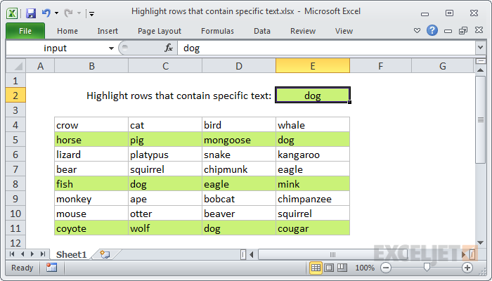
For example, assume you have a simple table of data in B4:E11 and you want to highlight all rows that contain the text "dog". Just select all data in the table and create a new conditional formatting rule that uses this formula:
=SEARCH("dog",$B4&$C4&$D4&$E4)
Note: with conditional formatting, the formula must be entered relative to the "active cell" in the selection, which is assumed to be B4 in this case.
Generic formula
=SEARCH(text,concatenated_text)
Explanation
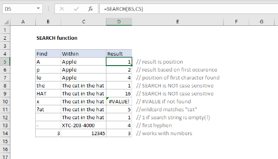
The SEARCH function returns the position of the text you are looking for as a number (if it exists). Conditional formatting automatically treats any positive number as TRUE, so the rule is triggered whenever SEARCH returns a number. When SEARCH doesn't find the text you're looking for, it returns a #VALUE error, which conditional formatting treats as FALSE.
Using the ampersand (&) we are concatenating all values in each row together and then searching the result with SEARCH. All addresses are entered in "mixed" format, with the columns locked and the rows left relative. Effectively, this means that all 4 cells in each row are tested with exactly the same formula.
Using other cells as inputs
Note that you don't have to hard-code any values that might change into the rule. Instead, you can use another cell as an "input" cell so you can easily change it later. For example, in this case, you could name cell E2 "input" and rewrite the formula like so:
=SEARCH(input,$B4&$C4&$D4&$E4)
You can then put any text value in E2, and the conditional formatting rule will respond instantly, highlighting rows that contain that text. See the video link below for a more detailed description.
Case sensitive option
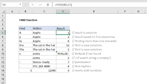
If you need a case-sensitive option, you can use the FIND function instead of SEARCH like so:
=FIND(input,$B4&$C4&$D4&$E4)
The FIND function works just like SEARCH but matches the case as well.