Highlight cells that end with

Note: Excel contains many built-in rules for highlighting values with conditional formatting, including a rule to highlight cells that end with specific text. However, if you want more flexibility, you can use your own formula, as explained in this article.

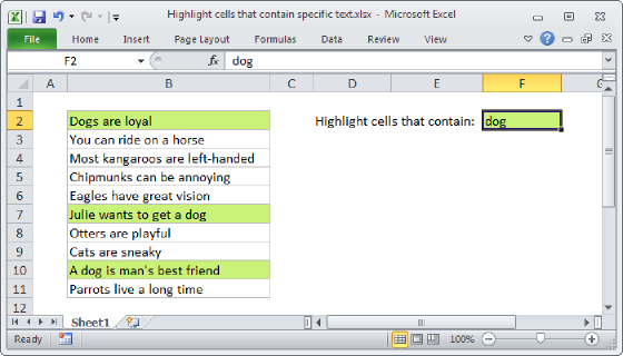
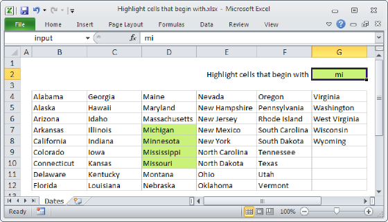
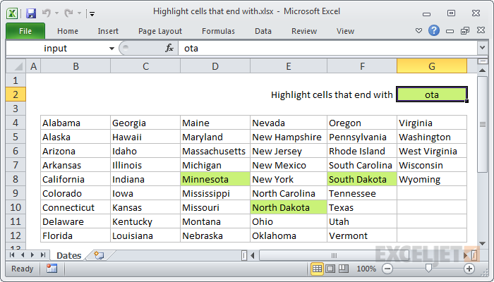
If you want to highlight cells that end with certain text, you can use a simple formula based on the COUNTIF function. For example, if you want to highlight states in the range B4:G12 that end with "ota", you can use:

=COUNTIF(B4,"*ota")

Note: with conditional formatting, it's important that the formula be entered relative to the "active cell" in the selection, which is assumed to be B4 in this case.

Explanation

When you use a formula to apply conditional formatting, the formula is evaluated relative to the active cell in the selection at the time the rule is created. In this case, the rule is evaluated for each cell in B4:G12, and the reference to B4 will change to the address of each cell being evaluated, since it is a relative address.

The formula itself uses the COUNTIF function to "count" cells that end with "ota" using the pattern "*ota" which uses a wildcard (*) to match any sequence of characters followed by "ota". From a practical standpoint, we are only counting 1 cell each time, which means we are either going to get back a 1 or a zero, which works perfectly for conditional formatting.

A simpler, more flexible rule using named ranges

By naming an input cell as a named range and referring to that name in the formula, you can make the formula more powerful and flexible. For example, if you name G2 "input", you can rewrite the formula like so:

=COUNTIF(B4,"*"&input)

This formula simply adds "*" to the beginning of whatever you put in the input cell. As a result, the conditional formatting rule will respond instantly whenever that value is changed.

Case sensitive option

COUNTIF is not case-sensitive, so if you need to check case as well, you can use a more complicated formula that relies on the RIGHT function together with EXACT:

=EXACT(RIGHT(A1,LEN(substring)),substring)

In this case, RIGHT extracts text from the right of each cell, and only the number of characters in the substring you are looking for, which is supplied by LEN. Finally EXACT compares the extracted text to the text you are looking for (the substring). EXACT is case-sensitive, so only will return TRUE when all characters match exactly.