Summary
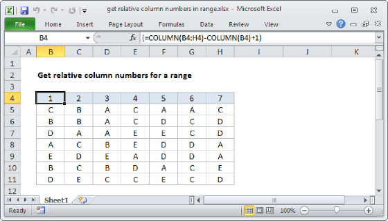
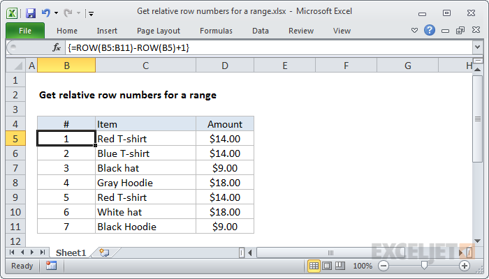
To get a full set of relative row numbers in a range, you can use an array formula based on the ROW function. In the example shown, the formula in B5:B11 is:
{=ROW(B5:B11)-ROW(B5)+1}
Note: this is an array formula that must be entered with Control + Shift + Enter. If you're entering this on the worksheet (and not inside another formula), make a selection that includes more than one row, enter the formula, and confirm with Control + Shift + Enter.
This formula will continue to generate relative numbers even when the range is moved. However, it's not a good choice if rows need to be sorted, deleted, or added because the array formula will prevent changes. The formula options explained here will work better.
Generic formula
{=ROW(range)-ROW(range.firstcell)+1}
Explanation
The first ROW function generates an array of 7 numbers like this:
{5;6;7;8;9;10;11}
The second ROW function generates an array with just one item like this:
{5}
which is then subtracted from the first array to yield:
{0;1;2;3;4;5;6}
Finally, 1 is added to get:
{1;2;3;4;5;6;7}
Generic version with named range
With a named range, you can create a more generic version of the formula using the MIN function or the INDEX function. For example, with the named range "list", you can use MIN like this:
{ROW(list)-MIN(ROW(list))+1}
With INDEX, we fetch the first reference in the named range, and using ROW on that:
{=ROW(list)-ROW(INDEX(list,1,1))+1}
You'll often see "relative row" formulas like this inside complex array formulas that need row numbers to calculate a result.
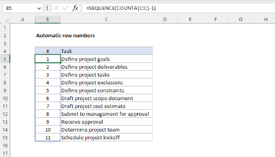
With SEQUENCE
With the SEQUENCE function the formula to return relative row numbers for a range is simple:
=SEQUENCE(ROWS(range))
The ROWS function provides the count of rows, which is returned to the SEQUENCE function. SEQUENCE then builds an array of numbers, starting with the number 1. So, following the original example above, the formula below returns the same result:
=SEQUENCE(ROWS(B5:B11)) // returns {1;2;3;4;5;6;7}
Note: the SEQUENCE formula is a new dynamic array function available only in Excel 365.