Filter this or that

To filter data to include only records where a value is this or that, you can use the FILTER function and simple boolean logic expressions. In the example shown, the formula in F5 is:

=FILTER(B5:D14,(D5:D14="red")+(D5:D14="blue"),"No results")

The result returned by FILTER includes only rows where group is "red" or "blue".

Explanation

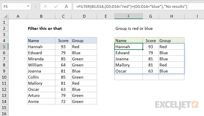
This formula relies on the FILTER function to retrieve data based on a logical test built with simple expressions and boolean logic:

(D5:D14="red")+(D5:D14="blue")

After each expression is evaluated, we have the following two arrays:

({TRUE;FALSE;FALSE;FALSE;FALSE;FALSE;TRUE;FALSE;FALSE;FALSE})+
({FALSE;TRUE;FALSE;FALSE;TRUE;FALSE;FALSE;TRUE;FALSE;FALSE})

The math operation (addition) coerces TRUE and FALSE values to 1s and 0s:

=({1;0;0;0;0;0;1;0;0;0})+({0;1;0;0;1;0;0;1;0;0})

The result is a single array like this:

={1;1;0;0;1;0;1;1;0;0}

This final array is delivered to the FILTER function as the include argument, and FILTER returns only rows that correspond to a 1. Or, to put it another way, FILTER removes rows that are zero.

Not mutually exclusive

In the example above, we are testing for two possible values in a single column of data. This means that the two tests are mutually exclusive — both tests can't return TRUE at the same time. However, if you are testing multiple columns/fields for values, there is the possibility that more than one logical test will return TRUE. In that case, the final array may contain numbers larger than 1 (i.e. TRUE + TRUE = 2). This makes a difference in some formulas. However, in this case, it doesn't matter, because FILTER will treat any non-zero value as TRUE when evaluating the include argument.

Video: Boolean algebra in Excel formulas