Explanation
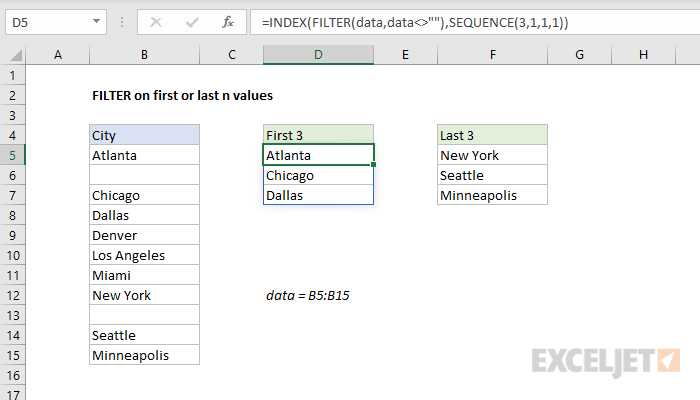
In this example, the goal is to extract the first 3 values or the last 3 values from the named range data (B5:B15). We also want to exclude any empty cells from our results. In the worksheet shown the formula in cell D5 is:
=INDEX(FILTER(data,data<>""),SEQUENCE(3,1,1,1))
Working from the inside out, we use the SEQUENCE function to construct a row number value for INDEX like this:
SEQUENCE(3,1,1,1)
We are asking SEQUENCE for an array of 3 rows x 1 column, starting at 1, with a step value of 1. The result is an array like this:
{1;2;3}
which is returned directly to the INDEX function as the row_num argument:
=INDEX(FILTER(data,data<>""),{1;2;3})
To construct the array for INDEX, we use the FILTER function to retrieve a list of non-blank entries from the named range data (B5:B15) like this:
FILTER(data,data<>"")
The array argument is data, and the include argument is the expression data<>"". This can be translated literally as "return values from the named range data where values in data are not empty". The result is an array with 9 values like this:
{"Atlanta";"Chicago";"Dallas";"Denver";"Los Angeles";"Miami";"New York";"Seattle";"Minneapolis"}
Notice values associated with the two empty cells have been removed. This array is returned to the INDEX function as its array argument.
Finally, INDEX returns the 1st, 2nd, and 3rd values from the array returned by FILTER:
{"Atlanta";"Chicago";"Dallas"}
Last n values
To get the last n values with FILTER, you use the same formula structure, with the inputs to SEQUENCE modified to construct a "last n" array of row numbers. For example, to get the last 3 non-blank values in the example shown, you can use a formula like this:
=INDEX(FILTER(data,data<>""),SORT(SEQUENCE(3,1,SUM(--(data<>"")),-1)))
The main trick here is counting the non-blank entries in the named range data like this:
SUM(--(data<>""))
We use a double-negative to force the TRUE FALSE values to 1s and 0s, then use the SUM function to get the count. The result is returned as the start argument inside SEQUENCE. We supply -1 for step to step backwards from start.
We also wrap the SORT function around SEQUENCE so the array returned is {7;8;9} and not {9;8;7}. This ensures that values are returned in the same order they appear in the source data.


