Filter contains one of many

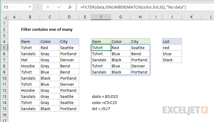
The FILTER function can filter data using a logical expression provided as the "include" argument. In this example, this argument is created with an expression that uses the ISNUMBER and MATCH functions like this:

=ISNUMBER(MATCH(color,list,0))

MATCH is configured to look for each color in C5:C15 inside the smaller range J5:J7. The MATCH function returns an array like this:

{1;#N/A;#N/A;#N/A;2;3;2;#N/A;#N/A;#N/A;3}

Notice numbers correspond to the position of "found" colors (either "red", "blue", or "black"), and errors correspond to rows where a target color was not found. To force a result of TRUE or FALSE, this array goes into the ISNUMBER function, which returns:

{TRUE;FALSE;FALSE;FALSE;TRUE;TRUE;TRUE;FALSE;FALSE;FALSE;TRUE}

The array above is delivered to the FLITER function as the include argument, and FILTER returns only rows that correspond to a TRUE value.

With hardcoded values

The example above is created with cell references, where target colors entered in the range J5:J7. However, but using an array constant, you can hardcode values into the formula like this with the same result:

=FILTER(data,ISNUMBER(MATCH(color,{"red","blue","black"},0)),"No data")