Dynamic named range with OFFSET

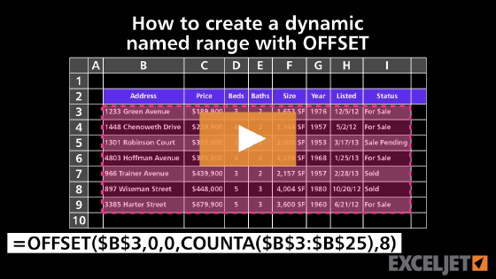
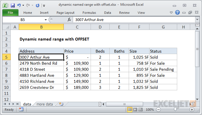
One way to create a dynamic named range with a formula is to use the OFFSET function together with the COUNTA function. Dynamic ranges are also known as expanding ranges - they automatically expand and contract to accommodate new or deleted data.

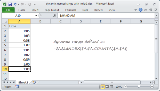
Note: OFFSET is a volatile function, which means it recalculates with every change to a worksheet. With a modern machine and smaller data set, this should't cause a problem but you may see slower performance on large data sets. In that case, consider building a dynamic named range with the INDEX function instead.

In the example shown, the formula used for the dynamic range is:

=OFFSET(B5,0,0,COUNTA($B$5:$B$100),COUNTA($B$4:$Z$4))

Note: this formula is meant to define a named range that can be used in other formulas.

Explanation

This formula uses the OFFSET function to generate a range that expands and contracts by adjusting height and width based on a count of non-empty cells.

The first argument in OFFSET represents the first cell in the data (the origin), which in this case is cell B5. The next two arguments are offsets for rows and columns, and are supplied as zero.

The last two arguments represent height and width. Height and width are generated on the fly by using COUNTA, which makes the the resulting reference dynamic.

For height, we use the COUNTA function to count non-empty values in the range B5:B100. This assumes no blank values in the data, and no values beyond B100. COUNTA returns 6.

For width, we use the COUNTA function to count non-empty values in the range B5:Z5. This assumes no header cells, and no headers beyond Z5. COUNTA returns 6.

At this point, the formula looks like this:

=OFFSET(B5,0,0,6,6)

With this information, OFFSET returns a reference to B5:G10, which corresponds to a range 6 rows height by 6 columns across.

Note: The ranges used for height and width should be adjusted to match the worksheet layout.

Variation with full column/row references

You can also use full column and row references for height and width like so:

=OFFSET($B$5,0,0,COUNTA($B:$B)-2,COUNTA($4:$4))

Note that height is being adjusted with -2 to take into account header and title values in cells B4 and B2. The advantage to this approach is the simplicity of the ranges inside COUNTA. The disadvantage comes from the huge size full columns and rows — care must be taken to prevent errant values outside the range, as they can easily throw off the count.

Determining the last row

There are several ways to determine the last row (last relative position) in a set of data, depending on the structure and content of the data in the worksheet: