Summary
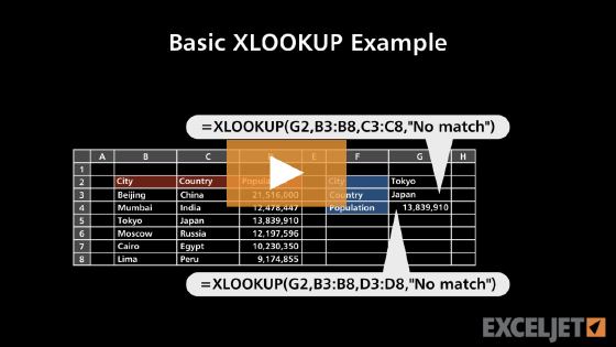
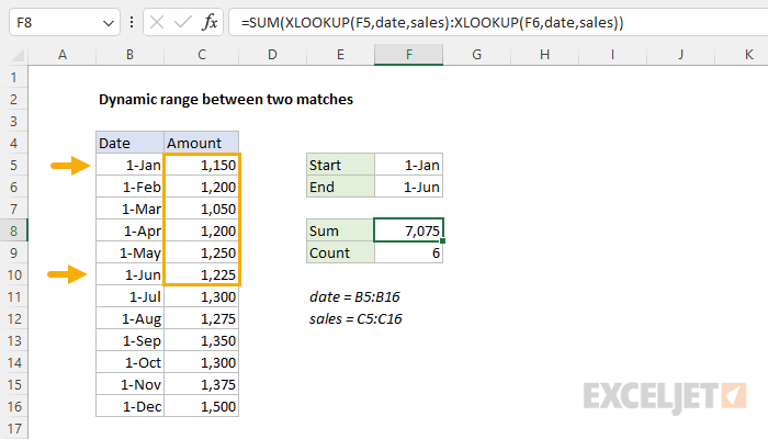
To create a dynamic range between two matches, you can use the XLOOKUP function. In the example shown, the formula in cell F8 is:
=SUM(XLOOKUP(F5,date,sales):XLOOKUP(F6,date,sales))
where date (B5:B16) and sales (C5:C16) are named ranges. The result is 7075, the sum of sales amounts between January 1 and June 1, inclusive.
Note: for the purpose of explanation, the worksheet above has just 12 rows of data. However, the same approach will work with a large set of data.
Generic formula
XLOOKUP(A1,range1,range2):XLOOKUP(A2,range1,range2)
Explanation
In this example, we have dates in B5:B16 and sales in C5:C16. Both ranges are named ranges. The goal is to create a dynamic range between two specific dates: the start date in cell F5 and the end date in cell F6. We then use a formula in F8 to sum the dynamic range, and a formula in F9 to count the dynamic range. In the current version of Excel, this problem can be easily solved with the XLOOKUP function. In older versions of Excel without XLOOKUP, you can use INDEX and MATCH. Both approaches are described below. This problem is a nice demonstration of how both XLOOKUP and INDEX return a valid reference that can be used like any other cell reference.
Range operator
One of Excel's most common operators is the colon (:), also known as a "range operator". The range operator (:) is used to construct ranges. For example, to create a reference from cell A1 to cell A9, you would use a range like this:
=A1:A9
To sum all values in this range, you would simply embed the range in the SUM function:
=SUM(A1:A9)
In this problem, we want to do essentially the same thing. However, the catch is that we want the range to be dynamic so that the references to A1 and A9 are the result of user input. Conceptually, the generic syntax for what we want looks like this:
=SUM(lookup1:lookup2)
In the code above, lookup1 should return a reference to the first cell in the range (the start date in F5), and lookup2 should be a reference to the last cell in the range (the end date in F6).
XLOOKUP function
The trick in solving this problem is to understand that the XLOOKUP function returns a reference and not just a value. This is not obvious in Excel, because even though XLOOKUP returns a reference, Excel will then immediately return the value at that reference. Nevertheless, the reference is there and can be used in other ways. In this case, we use this feature to assemble a range based on the results from two separate XLOOKUP formulas like this:
=SUM(XLOOKUP(F5,date,sales):XLOOKUP(F6,date,sales))
Inside the SUM function, notice we are using two separate XLOOKUP formulas joined with the range operator (:). The first XLOOKUP formula locates the start date in F5 in column B and returns a reference to the corresponding cell in column C:
XLOOKUP(F5,date,sales) // returns C5
With the lookup_value provided as F5, the lookup_array given as date (B5:B16), and the return_array given as sales (C5:C16), XLOOKUP matches January 1 in cell B5 and returns a reference to cell C5 as a result. The second XLOOKUP formula is configured in the same way, except the lookup_value is F6 (the end date):
XLOOKUP(F6,date,sales) // returns C10
With June 1 in cell F6, the result from XLOOKUP is a reference to C10. Putting this all together, the formula in F8 is evaluated by Excel like this:
=SUM(XLOOKUP(F5,date,sales):XLOOKUP(F6,date,sales))
=SUM(C5:C10)
=7075
When the dates in F5 or F6 are changed, XLOOKUP returns new references and the range is dynamically updated. The SUM then returns a new result. To count results instead of summing results, just replace the SUM function with the COUNT function. In the worksheet shown, the formula in cell F9 looks like this:
=COUNT(XLOOKUP(F5,date,sales):XLOOKUP(F6,date,sales))
For a detailed overview of XLOOKUP, see How to use the XLOOKUP function.
INDEX and MATCH
In older versions of Excel without the XLOOKUP function, this problem can be solved in the same way with an INDEX and MATCH that uses the same structure:
=SUM(INDEX(sales,MATCH(F5,date,0)):INDEX(sales,MATCH(F6,date,0)))
This works because the INDEX function, like XLOOKUP, returns a reference when the array provided to INDEX is a range. Notice the range operator (:) sits between two separate INDEX and MATCH formulas. The first INDEX and MATCH formula locates the date entered in F5 (January 1) in column B and returns a corresponding reference from the sales amounts in column C:
INDEX(sales,MATCH(F5,date,0)) // returns C5
The result is a reference to cell C5 since cell B5 contains January 1. The second INDEX and MATCH formula is the same, except that the lookup value comes from cell F6:
INDEX(sales,MATCH(F6,date,0)) // returns C10
The result is a reference to cell C10 since cell B10 contains June 1. Excel evaluates this formula in the same way as the XLOOKUP version above, with exactly the same result:
=SUM(INDEX(sales,MATCH(F5,date,0)):INDEX(sales,MATCH(F6,date,0)))
=SUM(C5:C10)
=7075
If the dates in F5 and F6 are changed, the INDEX and MATCH formulas return new references, and the range they create is dynamically updated. The SUM function then returns a new result. To count results instead of summing results, just replace the SUM function with the COUNT function:
=COUNT(INDEX(sales,MATCH(F5,date,0)):INDEX(sales,MATCH(F6,date,0)))
For a detailed overview of INDEX with MATCH see: How to use INDEX and MATCH.