Summary
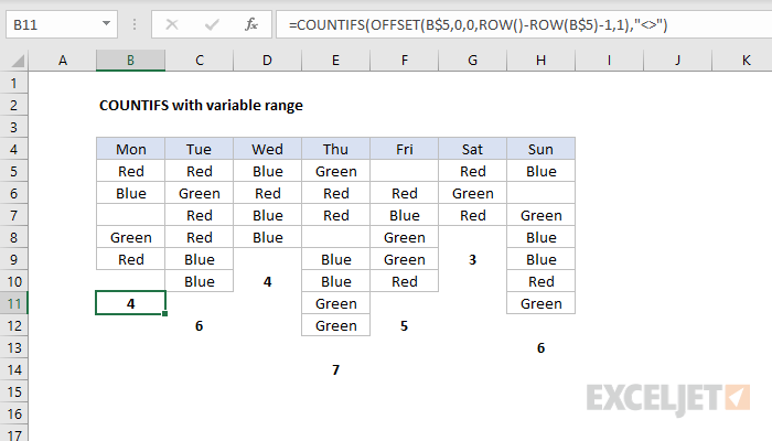
To configure COUNTIFS (or COUNTIF) with a variable range, you can use the OFFSET function. In the example shown, the formula in B11 is:
=COUNTIFS(OFFSET(B$5,0,0,ROW()-ROW(B$5)-1,1),"<>")
This formula counts non-blank cells in a range that begins at B5 and ends 2 rows above the cell where the formula lives. The same formula is copied and pasted 2 rows below the last entry in the data as shown.
Explanation
In the example shown, the formula in B11 is:
=COUNTIFS(OFFSET(B$5,0,0,ROW()-ROW(B$5)-1,1),"<>")
Working from the inside out, the work of setting up a variable range is done by the OFFSET function here:
OFFSET(B$5,0,0,ROW()-ROW(B$5)-1,1) // variable range
OFFSET has five arguments and is configured like this:
- reference = B$5, begin at cell B5, row locked
- rows = 0, offset zero rows from starting cell
- cols = 0, offset zero columns starting cell
- height = ROW()-ROW(B$5)-1 = 5 rows high
- width = 1 column wide
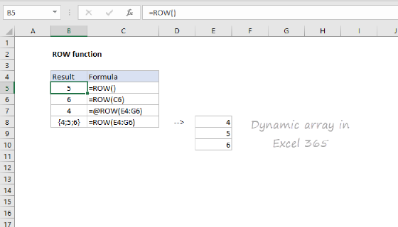
To work out the height of the range in rows, we use the ROW function like this:
ROW()-ROW(B$5)-1 // work out height
Since ROW() returns the row number of the "current" cell (i.e. the cell the formula lives in), we can simplify like this:
=ROW()-ROW(B$5)-1
=11-5-1
=5
With the above configuration, OFFSET returns the range B5:B9 directly to COUNTIFS:
=COUNTIFS(B5:B9,"<>") // returns 4
Notice the reference to B$5 in the above formula is a mixed reference, with the column relative and the row locked. This allows the formula to be copied to another column and still work. For example, once copied to C12, the formula is:
=COUNTIFS(OFFSET(C$5,0,0,ROW()-ROW(C$5)-1,1),"<>")
Note: OFFSET is a volatile function and can cause performance problems in large or complex worksheets.
With INDIRECT and ADDRESS
Another approach is to use a formula based on the INDIRECT and ADDRESS functions. In this case, we assemble a range as text, then use INDIRECT to evaluate the text as a reference. The formula in B11 would be:
=COUNTIFS(INDIRECT(ADDRESS(5,COLUMN())&":"&ADDRESS(ROW()-2,COLUMN())),"<>")
The ADDRESS function is used to construct a range like this:
ADDRESS(5,COLUMN())&":"&ADDRESS(ROW()-2,COLUMN())
In the first instance of ADDRESS, we supply row_number as the hardcoded value 5, and provide the column_number with the COLUMN function:
=ADDRESS(5,COLUMN()) // returns "$B$5"
In the second instance, we supply the "current" row_number minus 2, and the current column with the COLUMN function:
=ADDRESS(ROW()-2,COLUMN()) // returns "$B$9"
After concatenating these two values together, we have:
"$B$5:$B$9" // as text
Note this is a text string. To convert to a valid reference, we need to use INDIRECT:
=INDIRECT("$B$5:$B$9") // returns $B$5:$B$9 as valid range
Finally, the formula in B11 becomes:
=COUNTIFS($B$5:$B$9,"<>") // returns 4
Note: INDIRECT is a volatile function and can cause performance problems in large or complex worksheets.