Count visible columns

There is no direct way to detect a hidden column with a formula in Excel. You might think of using the SUBTOTAL function, but SUBTOTAL only works with vertical ranges. As a result, the approach described in this example is a workaround based on a helper formula that must be entered in a range that includes all columns in the scope of interest. In this example, this range is the named range "key".

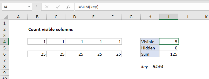
In the example shown, columns C and E are hidden. The helper formula, entered in B4 and copied across B4:F4, is based on the CELL function:

=CELL("width",B4)>0

The CELL function will only return a width for a cell in a visible column. When a column is hidden, the same formula will return zero. By checking if the result is greater than zero, we get a TRUE or FALSE result. The N function is used to coerce TRUE to 1 and FALSE to zero, so the final result is 1 when a column is visible, and 0 when a column is hidden. Nice.

To count visible columns, we use the SUM function formula in I4:

=SUM(key)

where "key" is the named range B4:F4.

Count hidden columns

To count hidden columns, the formula in I5 is:

=COLUMNS(key)-SUM(key)

The COLUMNS function returns the total columns in the range (5) and the SUM function returns the sum of visible columns (3), so the final result is 2:

=COLUMNS(key)-SUM(key)
=5-3
=2

With other operations

Once you have the "column key" in place, you can use it with other operations. For example, you could SUM values in visible columns by using SUM like this:

=SUM(key*B6:F6)

Although each cell in B6:F6 contains the number 25, SUM will return 75 when column C and E are hidden, as shown in the example.

Note: CELL function is a volatile function. Volatile functions normally recalculate with every worksheet change, so they can cause performance problems. Unfortunately, CELL does not fire when a column is hidden or made visible again. This means you will not see correct results until the worksheet recalculates, either with a normal change, or by pressing F9.