Summary
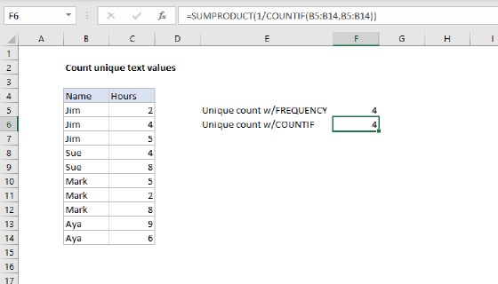
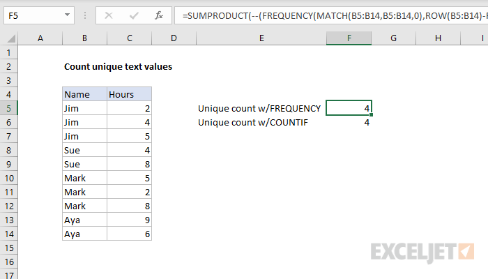
To count unique text values in a range, you can use a formula based on several functions: FREQUENCY, MATCH, ROW, and SUMPRODUCT. In the example shown, the formula in F5 is:
=SUMPRODUCT(--(FREQUENCY(MATCH(B5:B14,B5:B14,0),ROW(B5:B14)-ROW(B5)+1)>0))
which returns 4, since there are 4 unique names in B5:B14.
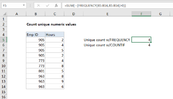
Note: Another way to count unique values is to use the COUNTIF function. This is a much simpler formula, but it can run slowly on large data sets.
In Dynamic Excel, you can use a simpler and faster formula based on UNIQUE.
Generic formula
=SUMPRODUCT(--(FREQUENCY(MATCH(data,data,0),ROW(data)-ROW(data.firstcell)+1)>0))
Explanation
This formula is more complicated than a similar formula that uses FREQUENCY to count unique numeric values because FREQUENCY doesn't normally work with non-numeric values. As a result, a large part of the formula simply transforms the non-numeric data into numeric data that FREQUENCY can handle.
Working from the inside out, the MATCH function is used to get the position of each item that appears in the data:
MATCH(B5:B14,B5:B14,0)
The result from MATCH is an array like this:
{1;1;1;4;4;6;6;6;9;9}
Because MATCH always returns the position of the first match, values that appear more than once in the data return the same position. For example, because "Jim" appears 3 times in the list, he shows up in this array 3 times as the number 1.
This array is fed into FREQUENCY as the data_array argument. The bins_array argument is constructed from this part of the formula:
ROW(B5:B14)-ROW(B5)+1)
which builds a sequential list of numbers for each value in the data:
{1;2;3;4;5;6;7;8;9;10}
At this point, FREQUENCY is configured like this:
FREQUENCY({1;1;1;4;4;6;6;6;9;9},{1;2;3;4;5;6;7;8;9;10})
FREQUENCY returns an array of numbers that indicate a count for each number in the data array, organized by bin. When a number has already been counted, FREQUENCY will return zero. This is a key feature in the operation of this formula. The result from FREQUENCY is an array like this:
{3;0;0;2;0;3;0;0;2;0;0} // output from FREQUENCY
Note: FREQUENCY always returns an array with one more item than the bins_array.
We can now rewrite the formula like this:
=SUMPRODUCT(--({3;0;0;2;0;3;0;0;2;0;0}>0))
Next, we check for values greater than zero (>0), which converts the numbers to TRUE or FALSE, then use a double-negative (--) to convert the TRUE and FALSE values to 1s and 0s. Now we have:
=SUMPRODUCT({1;0;0;1;0;1;0;0;1;0;0})
Finally, SUMPRODUCT simply adds the numbers up and returns the total, which in this case is 4.
Handling blank cells
Empty cells in the range will cause the formula to return an #N/A error. To handle empty cells, you can use a more complicated array formula that uses the IF function to filter out blank values:
{=SUM(IF(FREQUENCY(IF(data<>"", MATCH(data,data,0)),ROW(data)-ROW(data.firstcell)+1),1))}
Note: adding IF makes this into an array formula that requires control-shift-enter.
For more information, see this page.
From Mike Girvin's excellent book on array formulas, Control-Shift-Enter.
UNIQUE function in Excel 365
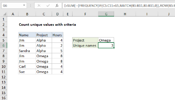
In Excel 365, the UNIQUE function provides a better, more elegant way to list unique values and count unique values. These formulas can be adapted to apply logical criteria.
A pivot table is also an excellent way to list and count unique values.