Summary
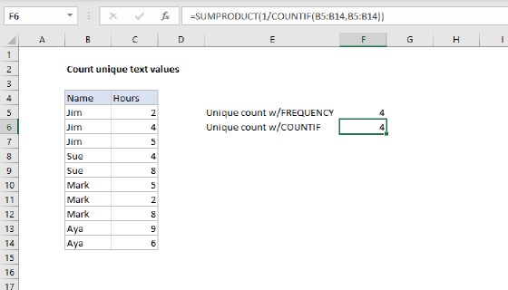
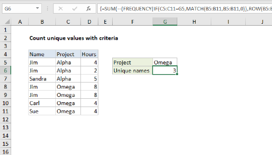
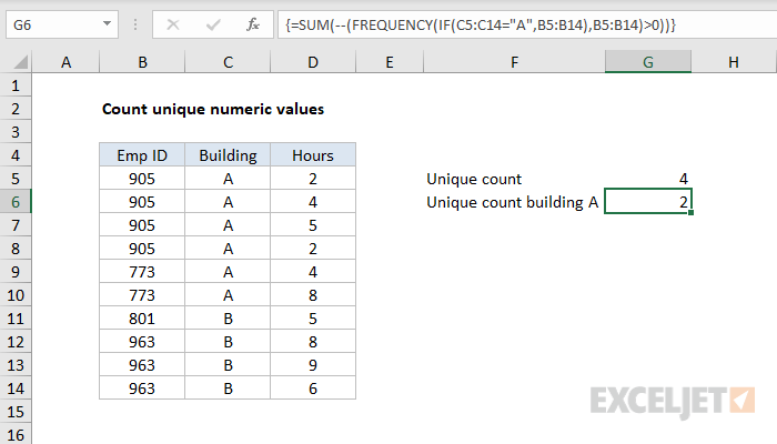
To count unique numeric values in a range, you can use a formula based on the FREQUENCY, SUM, and IF functions. In the example shown, employee numbers appear in the range B5:B14. The formula in G6 is:
=SUM(--(FREQUENCY(IF(C5:C14="A",B5:B14),B5:B14)>0))
which returns 2, since there are 2 unique employee ids in building A.
Note: this is an array formula and must be entered with control + shift + enter in Legacy Excel.
With Excel 365, you can use a simpler and faster formula based on UNIQUE.
Generic formula
{=SUM(--(FREQUENCY(IF(criteria,values),values)>0))}
Explanation
Note: Prior to Excel 365, Excel did not have a dedicated function to count unique values. This formula shows one way to count unique values, as long as they are numeric. If you have text values, or a mix of text and numbers, you'll need to use a more complicated formula.
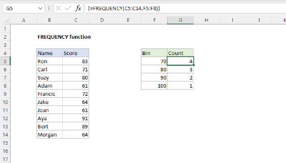
The Excel FREQUENCY function returns a frequency distribution, which is a summary table that contains the frequency of numeric values, organized in "bins". We use it here as a roundabout way to count unique numeric values. To apply criteria, we use the IF function.
Working from the inside-out, we first filter values with the IF function:
IF(C5:C14="A",B5:B14) // filter on building A
The result of this operation is an array like this:
{905;905;905;905;773;773;FALSE;FALSE;FALSE;FALSE}
Notice all ids in building B are now FALSE. This array is delivered directly to the FREQUENCY function as the data_array. For the bins_array, we supply the ids themselves:
FREQUENCY({905;905;905;905;773;773;FALSE;FALSE;FALSE;FALSE},{905;905;905;905;773;773;801;963;963;963})
With this configuration, FREQUENCY returns the array below:
{4;0;0;0;2;0;0;0;0;0;0}
The result is a bit cryptic, but the meaning is 905 appears four times, and 773 appears two times. The FALSE values are automatically ignored.
FREQUENCY has a special feature that automatically returns zero for any numbers that have already appeared in the data array, which is why values are zero once a number has been encountered. This is the feature that allows this approach to work.
Next, each of these values is tested to be greater than zero:
{4;0;0;0;2;0;0;0;0;0;0}>0
The result is an array like this:
{TRUE;FALSE;FALSE;FALSE;TRUE;FALSE;FALSE;FALSE;FALSE;FALSE;FALSE}
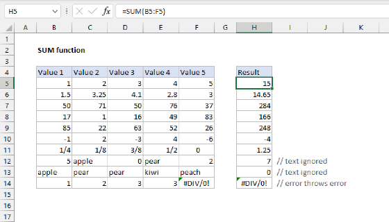
Each TRUE in the list represents a unique number in the list, and we just need to add up the TRUE values with SUM. However, SUM won't add up logical values in an array, so we need to first coerce the values into 1 or zero. This is done with the double-negative (--). The result is an array of only 1's or 0's:
{1;0;0;0;1;0;0;0;0;0;0}
Finally, SUM adds these values up and returns the total, which in this case is 2.
Multiple criteria
You can extend the formula to handle multiple criteria like this:
{=SUM(--(FREQUENCY(IF((criteria1)*(criteria2),values),values)>0))}
UNIQUE function in Excel 365
In Excel 365, the UNIQUE function provides a better, more elegant way to list unique values and count unique values. These formulas can be adapted to apply logical criteria.