Summary
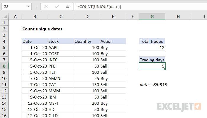
To count unique dates ("trading days" in the example) you can use the UNIQUE function with the COUNT function, or a formula based on the COUNTIF function. In the example shown, the formula in cell G8 is:
=COUNT(UNIQUE(date))
where date is the named range B5:B16.
Generic formula
=COUNT(UNIQUE(date))
Explanation
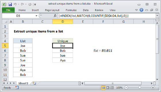
Traditionally, counting unique items with an Excel formula has been a tricky problem, because there hasn't been a dedicated unique function. However, that changed when dynamic arrays were added to Excel 365, along with several new functions, including UNIQUE.
Note: In older versions of Excel, you can count unique items with the COUNTIF function, or the FREQUENCY function, as explained below.
In the example shown, each row in the table represents a stock trade. On some dates, more than one trade is performed. The goal is to count trading days – the number of unique dates on which some kind of trade occurred. The formula in cell G8 is:
=COUNT(UNIQUE(date))
Working from the inside out, the UNIQUE function is used to extract a list of unique dates from the named range date:
UNIQUE(date) // extract unique values
The result is an array with 5 numbers like this:
{44105;44109;44111;44113;44116}
Each number represents an Excel date, without date formatting. The 5 dates are 1-Oct-20, 5-Oct-20, 7-Oct-20, 9-Oct-20, and 12-Oct-20.
This array is delivered directly to the COUNT function:
=COUNT({44105;44109;44111;44113;44116}) // returns 5
which returns a count of numeric values, 5, as the final result.
Note: The COUNT function counts numeric values, while the COUNTA function will count both numeric and text values. Depending on the situation, it may make sense to use one or the other. In this case, because dates are numeric, we use COUNT.
With COUNTIF
In an older version of Excel, you can use the COUNTIF function to count unique dates with a formula like this:
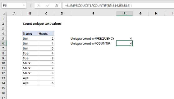
=SUMPRODUCT(1/COUNTIF(date,date))
Working from the inside out, COUNTIF returns an array with a count for every date in the list:
COUNTIF(date,date) // returns {2;2;3;3;3;2;2;2;2;3;3;3}
At this point, we have:
=SUMPRODUCT(1/{2;2;3;3;3;2;2;2;2;3;3;3})
After 1 is divided by this array, we have an array of fractional values:
{0.5;0.5;0.333333333333333;0.333333333333333;0.333333333333333;0.5;0.5;0.5;0.5;0.333333333333333;0.333333333333333;0.333333333333333}
This array is delivered directly to the SUMPRODUCT function. SUMPRODUCT then sums the items in the array and returns the total, 5.
With FREQUENCY
If you are working with a large set of data, you might have performance problems with the COUNTIF formula above. In that case, you can switch to an array formula based on the FREQUENCY function:
{=SUM(--(FREQUENCY(date,date)>0))}
Note: This is an array formula and must be entered with control + shift + enter, except in Excel 365.
This formula will calculate faster than the COUNTIF version above, but it will only work with numeric values. For more details, see this article.