Summary
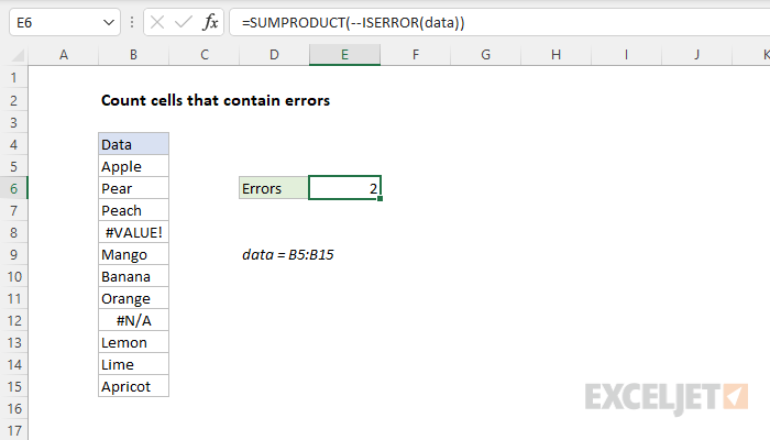
To count cells that contain errors, you can use the ISERRORfunction, wrapped in the SUMPRODUCT function. In the example shown, cell E6 contains this formula:
=SUMPRODUCT(--ISERROR(data))
Where data is the named range B5:B15.
Generic formula
=SUMPRODUCT(--ISERROR(range))
Explanation
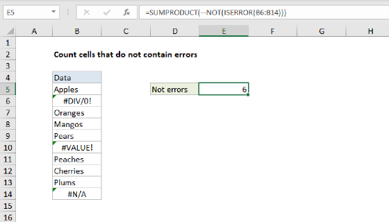
In this example, the goal is to count errors in the range B5:B15, which is named data for convenience. The article below explains several different approaches, depending on your needs. For background, this article: Excel Formula Errors.
COUNTIF function
One way to count individual errors is with the COUNTIF function like this:
=COUNTIF(data,"#N/A") // returns 1
=COUNTIF(data,"#VALUE!") // returns 1
=COUNTIF(data,"#DIV/0!") // returns 0
This is an odd syntax since technically errors are not text values. But COUNTIF is in a group of eight functions that have some quirks, and this is one of them. During calculation, COUNTIF is able to resolve the text into the given error and return a count of that error. One limitation of this approach is that there is no simple way to count all error types with a single formula. You might think we can use COUNTIF like this:
=COUNTIF(ISERROR(data),TRUE) // fails
The idea here is that the ISERROR function will return TRUE or FALSE, and COUNTIF will count the TRUE results. However, if you try to enter this formula, Excel won't let you. This is a case where COUNTIF won't work because it won't allow an "array operation" in place of a normal range. One solution is to use SUMPRODUCT with ISERROR, as explained below.
SUMPRODUCT function
A better way to count errors in a range is to use the SUMPRODUCT function with the ISERROR function and Boolean logic. The SUMPRODUCT function accepts one or more arrays, multiplies the arrays together, and returns the "sum of products" as a final result. If only one array is supplied, SUMPRODUCT simply returns the sum of items in the array. In the example shown, the formula in E6 is:
=SUMPRODUCT(--ISERROR(data))
Working from the inside out, the ISERROR function returns TRUE when a cell contains an error, and FALSE if not. Because there are eleven cells in the range B5:B15, ISERROR evaluates each cell and returns 11 results in an array like this:
{FALSE;FALSE;FALSE;TRUE;FALSE;FALSE;FALSE;TRUE;FALSE;FALSE;FALSE}
Next, we use a double negative (--) to convert the TRUE and FALSE values to 1s and 0s. The resulting array inside the SUMPRODUCT function looks like this:
=SUMPRODUCT({0;0;0;1;0;0;0;1;0;0;0})
Finally, SUMPRODUCT sums the items in this array and returns the total, which is 2 in this case.
ISERR option
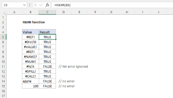
The ISERROR function counts all errors. If for some reason you want to count all errors except #N/A, you can use the ISERR function instead:
=SUMPRODUCT(--ISERR(data)) // returns 1
Since one of the errors shown in the example is #N/A, this formula returns 1 instead of 2.
Count by error code
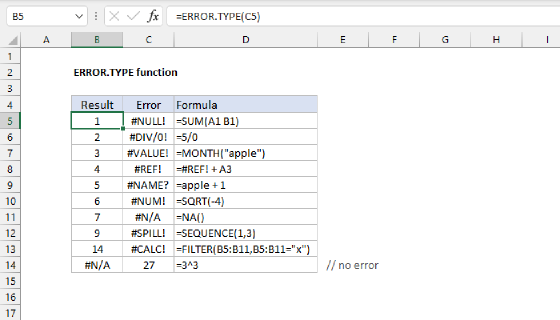
Each Excel formula error is associated with a numeric error code (complete list here). You can retrieve this code with the ERROR.TYPE function. To count errors by numeric code, you can use ERROR.TYPE instead of ISERROR. For example to count #VALUE! errors, which have a numeric code of 3, you can use a formula like this:
=SUMPRODUCT(--(IFERROR(ERROR.TYPE(data),0)=3))
In an ironic twist, we need the IFERROR function to help us here. The ERROR.TYPE function will return a numeric code for any formula error. However, if a cell does not contain an error, ERROR.TYPE itself returns an #N/A error, which will bubble to the top and cause the entire formula to return #N/A. We use IFERROR to map the #N/A errors to zero so that we can compare the results from ERROR.TYPE to 3 without trouble. This part of the formula evaluates like this:
=IFERROR(ERROR.TYPE(data),0)=3)
=IFERROR({#N/A;#N/A;#N/A;3;#N/A;#N/A;#N/A;7;#N/A;#N/A;#N/A},0)=3)
={0;0;0;3;0;0;0;7;0;0;0}=3
={FALSE;FALSE;FALSE;TRUE;FALSE;FALSE;FALSE;FALSE;FALSE;FALSE;FALSE}
Notice in the second step above, we see error code 3 and error code 7. This indicates the #VALUE! and #N/A error in data (B5:B15). After IFERROR runs, the #N/A errors are gone and replaced with zeros, as you can see in the third step. This lets us check for error code 3 without trouble. From there, we use a double negative to convert the TRUE and FALSE values to 1s and 0s and the resulting array is returned directly to SUMPRODUCT:
=SUMPRODUCT({0;0;0;1;0;0;0;0;0;0;0}) // returns 1
The final result is 1, since there is one error in data with an error code of 3.
Note: In Excel 365 and Excel 2021 you can use the SUM function instead of SUMPRODUCT in all formulas above if you prefer, with some caveats. This article provides a complete explanation.