Summary
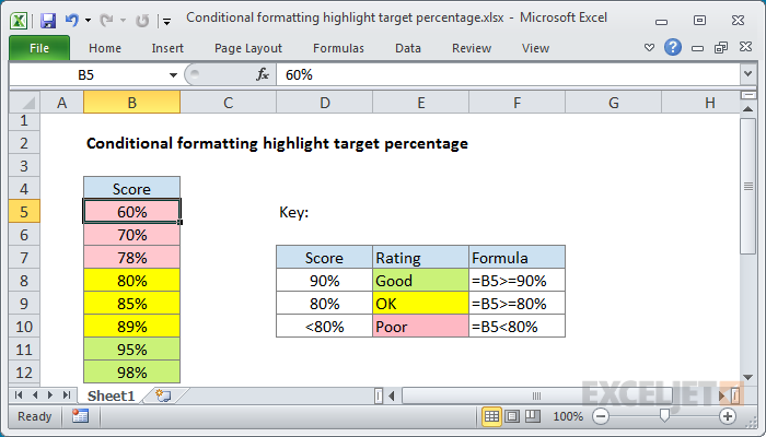
To highlight a percentage value in a cell using different colors, where each color represents a particular level, you can use multiple conditional formatting rules, with each rule targeting a different threshold. In the example shown, conditional formatting is applied to the range B5:B12 using 3 formulas:
=B5>=90% // green
=B5>=80% // yellow
=B5<80% // pink
Note: formulas are entered relative to the upper left cell in the range, which is B5 in this example.
Generic formula
=A1>=X
=A1>=Y
=A1<Y
Explanation
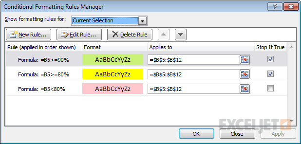
Conditional formatting rules are evaluated in order.
- For each cell in the range B5:B12, the first formula is evaluated. If the value is greater than or equal to 90%, the formula returns TRUE and the green fill is applied. If the value is not greater than or equal to 90%, the formula returns FALSE and the rule is not triggered.
- For each cell in the range B5:B12, the second formula is evaluated. If the value is greater than or equal to 80%, the formula returns TRUE and the yellow fill is applied.
- For each cell in the range B5:B12, the third formula is evaluated. If the value is less than 80%, the formula returns TRUE and the pink fill is applied.
The "stop if true" option is enabled for the first two rules to prevent further processing, since the rules are mutually exclusive.