Summary
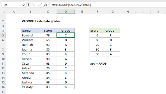
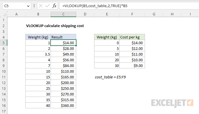
This example shows how to use the VLOOKUP function to calculate the total shipping cost for an item in one formula, where the cost per kilogram (kg) varies according to weight. This requires an "approximate match" since in most cases the actual weight will not appear in the shipping cost table. The formula in cell C5 is:
=VLOOKUP(B5,cost_table,2,TRUE)*B5
where cost_table (E5:F9) is a named range. In cell C5, the formula returns $14.00, the correct cost to ship an item that weighs 1 kilogram. As the formula is copied down, a cost is returned for each weight in the list.
Generic formula
=VLOOKUP(weight,cost_table,column,TRUE)*weight
Explanation
This example shows how to use the VLOOKUP function to calculate the total shipping cost for an item in one formula, where the cost per kilogram (kg) varies according to weight. This requires an "approximate match" since in most cases the actual weight will not appear in the shipping cost table. For convenience, the range E5:F9 is named cost_table. This is an "approximate-match" lookup problem because it is not likely that a given weight will be found in the cost table. As a result, the formula needs to match the largest weight in the table that is less than or equal to the given weight. Finally, the result of the lookup operation should multiply the cost per kilogram returned by VLOOKUP by the weight in column B to get a final cost.
VLOOKUP function
VLOOKUP is an Excel function to get data from a table organized vertically. Lookup values must appear in the first column of the table provided to VLOOKUP, and the information to retrieve is specified by column number. If you are new to VLOOKUP, see:
- How to use VLOOKUP - overview with examples and video links
VLOOKUP solution
In the worksheet shown, the formula in cell C5 is:
=VLOOKUP(B5,cost_table,2,TRUE)*B5
where cost_table (E5:F9) is a named range. VLOOKUP requires lookup values to be in the first column of the lookup table. To retrieve the correct cost per kilogram for a given weight, VLOOKUP is configured like this:
- The lookup_value comes from cell B5
- The table_array is the named range cost_table (E5:F9)
- The col_index_num is 2 since the cost appears in the second column of the table
- The range_lookup argument is set to TRUE = approximate match
With a score provided as a lookup value, VLOOKUP will scan the first column of the table. If it finds an exact match, it will return the cost in that row. If VLOOKUP does not find an exact match, it will continue scanning until it finds a value greater than the lookup value, then it will "step back", and return the cost in the previous row. As the formula is copied down column C, the VLOOKUP function looks up each weight in column B and returns the correct cost per kilogram (kg). Finally, the result from VLOOKUP is multiplied by the original weight in column B to get a total shipping cost.
Notes: (1) In approximate match mode, VLOOKUP assumes the table is sorted by the values in the first column. This means the cost table must be sorted in ascending order by weight. (2) As an alternative, you could add a helper column that contains only the VLOOKUP part of the formula to calculate the cost per kilogram, then perform the multiplication separately.
Named range optional
The named range in this example is optional and used for convenience only because it makes the formula easier to read and means that the cost table does not need to be locked when the formula is copied down column C. To avoid using a named range, use an absolute reference like this:
=VLOOKUP(B5,$E$5:$F$9,2,TRUE)*B5
VLOOKUP match modes
VLOOKUP has two match modes: exact match and approximate match, controlled by an optional fourth argument called range_lookup. When range_lookup is omitted, it defaults to TRUE and VLOOKUP performs an approximate match. This means we could leave out the range_lookup and get the same result with this formula:
=VLOOKUP(B5,cost_table,2)*B5
However, I recommend that you always provide a value for range_lookup because it makes you consider the behavior you want. In other words, giving a value for range_lookup acts as a reminder to you and others of the intended behavior.
Notes: If the weight is less than the first entry in the table, VLOOKUP will return the #N/A error. In the example shown, we use zero in cell E5 to make sure this does not occur.
Adding a minimum cost
To modify the formula to return a minimum cost of $15, regardless of weight, you can nest the original formula inside the MAX function like so:
=MAX(VLOOKUP(B5,cost_table,2,TRUE)*B5,15)
After the original formula runs and returns a calculated total cost, the MAX function will return whichever is greater - the result of the formula or 15.