Summary
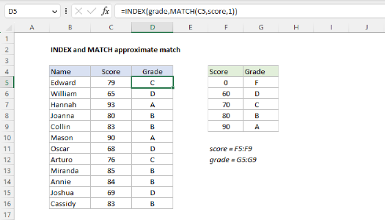
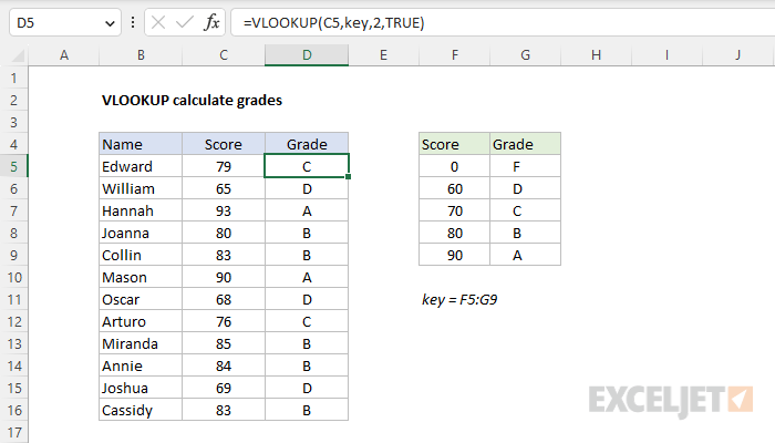
This example shows how to use the VLOOKUP function to calculate the correct grade for a given score using a table that holds the thresholds for each available grade. This requires an "approximate match" since in most cases the actual score will not exist in the table. The formula in cell D5 is:
=VLOOKUP(C5,key,2,TRUE)
where key (F5:G9) is a named range. In cell D5, the formula returns "C", the correct grade for a score of 79. As the formula is copied down, a grade is returned for each score in the list.
Generic formula
=VLOOKUP(score,key,2,TRUE)
Explanation
In this example, the goal is to calculate the correct grade for each name in column B using the score in column C and the table in F5:G9 as a "key" to assign grades. For convenience only, the range F5:G9 has been named key. This is a classic "approximate-match" lookup problem because it is not likely that a given score will be found in the lookup table. The desired behavior is to match the largest value in the table that is less than or equal to the score. In this way, the table acts to group scores into buckets, where each bucket is a particular grade.
VLOOKUP function
VLOOKUP is an Excel function to get data from a table organized vertically. Lookup values must appear in the first column of the table provided to VLOOKUP, and the information to retrieve is specified by column number. For a complete introduction to VLOOKUP with many examples and video links see:
- How to use VLOOKUP - overview with examples and video
VLOOKUP solution
In the worksheet shown, the formula in cell D5 is:
=VLOOKUP(C5,key,2,TRUE)
VLOOKUP requires lookup values to be in the first column of the lookup table. To retrieve the correct grade for any given score, VLOOKUP is configured like this:
- The lookup_value comes from cell C5
- The table_array is the named range key (F5:G9)
- The col_index_num is 2 since grades are in the second column
- The range_lookup argument is set to TRUE = approximate match
In approximate match mode, VLOOKUP assumes the table is sorted by the values in the first column. With a score provided as a lookup value, VLOOKUP will scan the first column of the table. If it finds an exact match, it will return the grade in that row. If VLOOKUP does not find an exact match, it will continue scanning until it finds a value greater than the lookup value, then it will "step back", and return the grade in the previous row. As the formula is copied down column D, the VLOOKUP function looks up each score in column C and returns the correct grade in column D
Named range optional
The named range in this example is optional and used for convenience only because it makes the formula easier to read and means that the tax rate does not need to be locked. To avoid using a named range, use an absolute reference like this:
=VLOOKUP(C5,$F$5:$G$9,2,TRUE)
VLOOKUP match modes
VLOOKUP has two match modes: exact match and approximate match, controlled by an optional fourth argument called range_lookup. When range_lookup is omitted, it defaults to TRUE and VLOOKUP performs an approximate match. This means we could leave out the range_lookup and get the same result with this formula:
=VLOOKUP(C5,key,2)
However, I recommend you always provide a value for range_lookup because it forces you to consider what you want. Providing a value for range_lookup acts as a reminder to you and others of the intended behavior.
Notes: (1) If the score is less than the first entry in the table, VLOOKUP will return the #N/A error. In the example shown, we use zero in cell F5 to make sure this does not occur. (2) You can use INDEX and MATCH to solve this same problem.