Summary
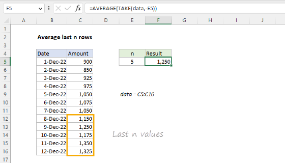
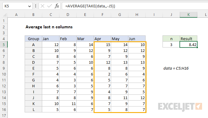
To average the last n columns in a set of data, you can use the TAKE function with the AVERAGE function. In the example shown, the formula in K5 is:
=AVERAGE(TAKE(data,,-J5))
where data is the named range C5:H16 and n is entered in cell J5 as a variable. The result is 8.42, the average of values in the range F5:H16.
Notes: (1) The TAKE function is new in Excel. See below for options that will work in older versions. (2) The example shows an average across 12 rows, but the formula will work fine with a single row of data.
Generic formula
=AVERAGE(TAKE(data,,-n))
Explanation
In this example, the goal is to average the last n columns in a set of data, where n is a variable entered in cell K5 that can be changed at any time. Since more data may be added, a key requirement is to average amounts by position. For convenience, the values to average are in the named range data (C5:H16). In the latest version of Excel, the best way to solve this problem is with the TAKE function, a new dynamic array function in Excel. In Legacy Excel, you can use the OFFSET function or the INDEX function. All three approaches are explained below.
TAKE function
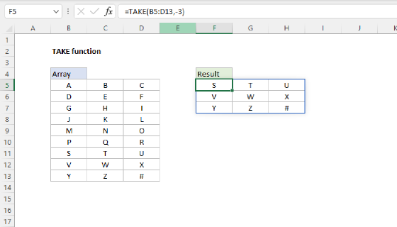
The TAKE function returns a subset of a given array or range. The size of the array returned is determined by separate rows and columns arguments:
=TAKE(array,rows,columns)
When positive numbers are provided for rows or columns, TAKE returns values from the start of the array:
=TAKE(array,3) // get first 3 rows
=TAKE(array,,3) // get first 3 columns
When negative numbers are provided, TAKE returns values from the end of the array:
=TAKE(array,-3) // get last 3 rows
=TAKE(array,,-3) // get last 3 columns
In the worksheet shown, data is the named range C5:H16. We can retrieve the last 3 columns like this:
=TAKE(data,,-3) // last 3 columns
Notice we simply omit rows in this case because we want all rows in data*.* To make the number of columns variable, we simply swap in the reference to J5 and add a negative sign:
=TAKE(data,,-J5)
Finally, to average the result from TAKE, we nest the TAKE function inside the AVERAGE function:
=AVERAGE(TAKE(data,,-J5))
With 3 in cell J5, TAKE returns the last 3 columns in data. This result is handed off to the AVERAGE function, which returns a final result of 8.42, the average of values in the range F5:H16.
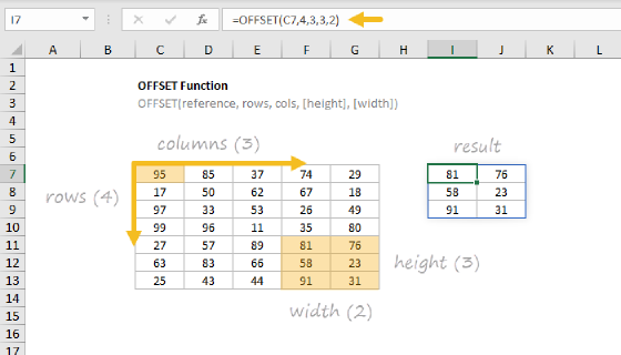
OFFSET function
In older versions of Excel, another way to solve this problem is to use the OFFSET function. The OFFSET function returns a reference to a range constructed with five inputs: (1) a starting point, (2) a row offset, (3) a column offset, (4) a height in rows, (5) a width in columns. To average the last 3 columns in the named range data, we can use the OFFSET function like this:
=AVERAGE(OFFSET(data,0,COLUMNS(data)-J5,,J5))
Inside the OFFSET function, we provide data for reference and 0 for rows, since we don't want any row offset. Next, we count the number of columns in data with the COLUMNS function and subtract the value for n in cell J5 to get a value for cols, the column offset. We leave height empty, because OFFSET will automatically inherit the height of reference, and we supply J5 for width since we want a 3-column range in the end. In this configuration, OFFSET returns a 3-column range starting at cell F5 in data containing all 12 rows.
Note: the OFFSET function is a volatile function and can cause performance problems in larger or more complicated worksheets. If you run into this problem, see the INDEX solution below.
INDEX function
Another way to solve this problem is to use the versatile INDEX function in a formula like this:
=AVERAGE(INDEX(data,0,COLUMNS(data)-(J5-1)):INDEX(data,0,COLUMNS(data)))
The key to understanding this formula is to realize that the INDEX function can return a reference to entire rows and entire columns. To generate a reference to the "last n columns" in a table, we build a reference in two parts: the left column and the right column, then use the range operator (:) to join the two parts together:
=AVERAGE(left:right)
To get a reference to the left column, we use:
INDEX(data,0,COLUMNS(data)-(J5-1))
Since data contains 6 columns, the COLUMNS function returns 6, and this simplifies to:
INDEX(data,0,4) // column 4
INDEX returns a reference to column 4, F5:F16. For the right column in the range, we use INDEX like this:
INDEX(data,0,COLUMNS(data))
Since COLUMNS returns 6, this simplifies to:
INDEX(data,0,6) // column 6
INDEX returns a reference to column 6, H5:H16. Together, the two INDEX functions return a reference to columns 4 through 6 in the data (i.e. F5:H16). The range operator (:) joins the two references together, and the AVERAGE function returns a final result of 8.42.