Explanation
The ADDRESS function creates a reference based on a given row and column number. In this case, we want to get the first row and the first column used by the named range data (B5:D14). To get the first row used, we use the ROW function together with the MIN function like this:
MIN(ROW(data))
Because data contains more than one row, ROW returns an array of row numbers:
{5;6;7;8;9;10;11;12;13;14}
This array goes directly to the MIN function, which returns the smallest number:
MIN({5;6;7;8;9;10;11;12;13;14}) // returns 5
To get the first column, we use the COLUMN function in the same way:
MIN(COLUMN(data))
Since data contains three rows, COLUMN returns an array with three column numbers:
{2,3,4}
and the MIN function again returns the smallest number:
MIN({2,3,4}) // returns 2
Both results are returned directly to the ADDRESS function, which constructs a reference to the cell at row 5, column 2:
=ADDRESS(5,2) // returns $B$5
If you want a relative address instead of an absolute reference, you can supply 4 for the third argument like this:
=ADDRESS(MIN(ROW(data)),MIN(COLUMN(data)),4) // returns B5
CELL function alternative
Although it's not obvious, the INDEX function returns a reference, so we can use the CELL function with INDEX to get the address of the first cell in a range like this:
=CELL("address",INDEX(data,1,1))
In this case, we use the INDEX function to get a reference to the first cell in the range by giving INDEX 1 for row number and 1 for column number, with data for array:
INDEX(data,1,1) // returns reference to B5
INDEX then returns a reference to cell B5, and we use the CELL function with "address", to display the address.
Note: The CELL function is a volatile function that can cause performance problems in large or complex workbooks.


