Purpose
Sum of squares of differences in two arrays
Return value
Calculated sum of squares of differences
Syntax
=SUMXMY2(array_x, array_y)- array_x - The first range or array containing numeric values.
- array_y - The second range or array containing numeric values.
Using the SUMXMY2 function
The Excel SUMXMY2 function returns the sum of squares of differences between corresponding values in two arrays. The "m" in the function name stands for "minus", as in "sum x minus y squared".
SUMXMY2 takes two arguments, array_x and array_y. Array_x is the first range or array or range of numbers, and array_y is the second range or array of numbers. Both arguments can be provided as an array constant or as a range.
Examples
=SUMXMY2({0,1},{1,2})// returns 2
=SUMXMY2({1,2,3},{1,2,3}) // returns 0
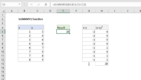
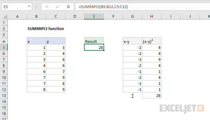
In the example shown above, the formula in E5 is:
=SUMXMY2(B5:B12,C5:C12)
which returns 28 as a result.
Equation
The equation used to calculate the sum of squares is:
This formula can be created manually in Excel with the exponentiation operator (^) like this:
=SUM((range1-range2)^2)
With the example as shown, the formula below will return the same result as SUMX2MY2:
=SUM((B5:B12-C5:C12)^2) // returns 28
Notes
- Arguments can be a mix of constants, names, arrays, or references that contain numbers.
- Text values are ignored, but cells with zero values are included.
- SUMXMY2 returns #N/A if the arrays contain different numbers of cells.