Excel MAXIFS function

The Excel MAXIFS function returns the largest numeric value in cells that meet multiple conditions, referred to as criteria. To define criteria, MAXIFS supports logical operators (>,<,<>,=) and wildcards (*,?,~), and can apply conditions to cells that contain dates, numbers, and text.

Purpose

Get maximum value with criteria

Return value

Maximum value

Syntax

=MAXIFS(max_range,range1,criteria1,[range2],[criteria2],...)

max_range - Range of values used to determine maximum.
range1 - The first range to evaluate.
criteria1 - The criteria to use on range1.
range2 - [optional] The second range to evaluate.
criteria2 - [optional] The criteria to use on range2.

Using the MAXIFS function

The MAXIFS function returns the largest numeric value in cells that meet multiple conditions, referred to as criteria. Each condition is provided with a separate range and criteria. To define criteria, MAXIFS supports various logical operators (>,<,<>,=) and wildcards (*,?,~). The syntax used to apply criteria in MAXIFS is a bit tricky because it is unusual in Excel. See below for details.

Key features

Can handle up to 126 conditions.
Each new condition requires a separate range and criteria.
To be included in the final result, all conditions must be TRUE.
Returns zero (0) when no cells meet the supplied criteria.
Automatically ignores empty cells that meet supplied criteria.
Returns a #VALUE! error if criteria_range is not the same size as max_range.

Unlike most other Excel functions, MAXIFS requires an actual range for max/criteria ranges. If you try to use an array, Excel will not let you enter the formula.

Syntax

The syntax for the MAXIFS function depends on the criteria being evaluated. Each condition is provided with a separate range and criteria. The generic syntax for MAXIFS looks like this:

=MAXIFS(max_range,range1,criteria1) // 1 condition
=MAXIFS(max_range,range1,criteria1,range2,criteria2) // 2 conditions

The MAXIFS function takes three required arguments: max_range, range1, and criteria1. With these three arguments, MAXIFS returns the maximum number in max_range where corresponding cells in range1 meet the condition set by criteria1. Additional conditions are applied using range/criteria pairs. The second condition is defined by range2 and criteria2, the third condition is range3 and criteria3, and so on. MAXIFS can handle up to 126 range/criteria pairs.

Criteria

The MAXIFS function supports logical operators (>,<,<>,=) and wildcards (*,?) for partial matching. Because MAXIFS is in a group of eight functions that split logical criteria into two parts, the syntax is a bit tricky. Each condition requires a separate range and criteria, and operators need to be enclosed in double quotes (""). The table below shows some common examples:

Target	Criteria
Cells greater than 75	">75"
Cells equal to 100	100 or "100"
Cells less than or equal to 100	"<=100"
Cells equal to "Red"	"red"
Cells not equal to "Red"	"<>red"
Cells that are blank ""	""
Cells that are not blank	"<>"
Cells that begin with "X"	"x*"
Cells less than A1	"<"&A1
Cells less than today	"<"&TODAY()

Notice the last two examples use concatenation with the ampersand (&) character. When a criteria argument includes a value from another cell, or the result of a formula, logical operators like "<" must be joined with concatenation. This is because Excel needs to evaluate cell references and formulas first to get a value before that value can be joined to an operator.

Basic Example

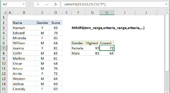
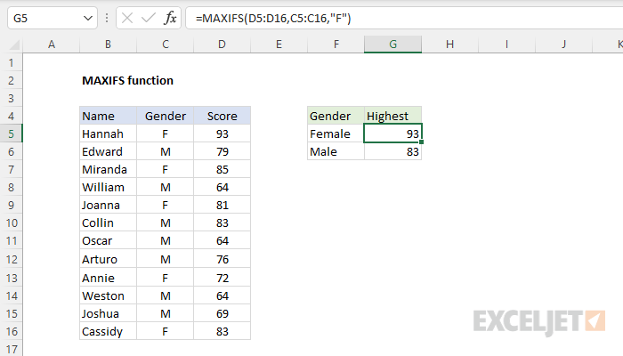
In the worksheet shown above, the formulas in G5 and G6 are:

=MAXIFS(D5:D16,C5:C16,"F") // returns 93
=MAXIFS(D5:D16,C5:C16,"M") // returns 83

In the first formula, MAXIFS returns the maximum value in D5:D16 where C5:C16 is equal to "F" (93). In the second formula, MAXIFS returns the maximum value in D5:D16 where C5:C16 is equal to "M" (83).

Two criteria

In the example below, the MAXIFS function is used with two criteria, one for Gender and one for Group. Note conditions are added in range/criteria pairs. The range E5:E16 is paired with the condition "B".

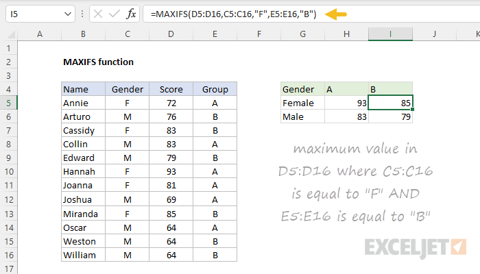
Example of MAXIFS function with two criteria

The formulas in H5:I6 are:

H5=MAXIFS(D5:D16,C5:C16,"F",E5:E16,"A") // returns 93
I5=MAXIFS(D5:D16,C5:C16,"F",E5:E16,"B") // returns 85
H6=MAXIFS(D5:D16,C5:C16,"M",E5:E16,"A") // returns 83
I6=MAXIFS(D5:D16,C5:C16,"M",E5:E16,"B") // returns 79

Other criteria

To return the maximum value in A1:A100 when cells in B1:B100 are greater than 50:

=MAXIFS(A1:A100,B1:B100,">50")

To get the maximum value in A1:A100 when cells in B1:B100 are less than or equal to 100, and cells in C1:C100 are greater than zero:

=MAXIFS(A1:A100,B1:B100,"<=100",C1:C100,">0")

Not equal to

To construct "not equal to" criteria, use the "<>" operator surrounded by double quotes (""). For example, to return the maximum value in A1:A100 when cells in B1:B100 are not equal to "red":

=MAXIFS(A1:A100,B1:B100,"<>red")

Value from another cell

When using a value from another cell in a condition, the cell reference must be concatenated to the operator. For example, to return the maximum value in A1:A100 when cells in B1:B100 are greater than the value in C1:

=MAXIFS(A1:A100,B1:B100,">"&C1)

Notice the greater than operator (>) is enclosed in quotes (""), but the cell reference (C1) is not.

Wildcards

The wildcard characters question mark (?), asterisk(*), or tilde (~) can be used in criteria. A question mark (?) matches any one character, and an asterisk (*) matches zero or more characters. For example, to return the maximum value in A1:A100 when cells in B1:B100 begin with "a":

=MAXIFS(A1:A100,B1:B100,"a*")

The tilde (~) is an escape character to allow you to find literal wildcards. For example, to match a literal question mark (?), asterisk(*), or tilde (~), add a tilde in front of the wildcard (i.e. ~?, ~*, ~~).

Notes

Conditions are applied using range/criteria pairs.
MAXIFS will return a #VALUE error if any criteria range is not the same size as max_range.
If no criteria match, MAXIFS will return zero (0).
MAXIFS ignores empty cells that meet criteria.