Summary
If VLOOKUP finds more than one match, will you get the first match or the last match? It's a trick question. It depends :) This article explains this confusing topic in detail, with lots of examples.
In the current version of Excel you can use the FILTER function to get all matches and the XLOOKUP function to get the last match only. Depending on your needs, FILTER might be a better option than the first or last match.
One of the more confusing aspects of lookup functions in Excel is understanding how to get the first or last match in a set of data with more than one match. This is because Excel's behavior changes depending on (1) whether you are performing an exact or approximate match, and (2) whether the data is sorted or not.
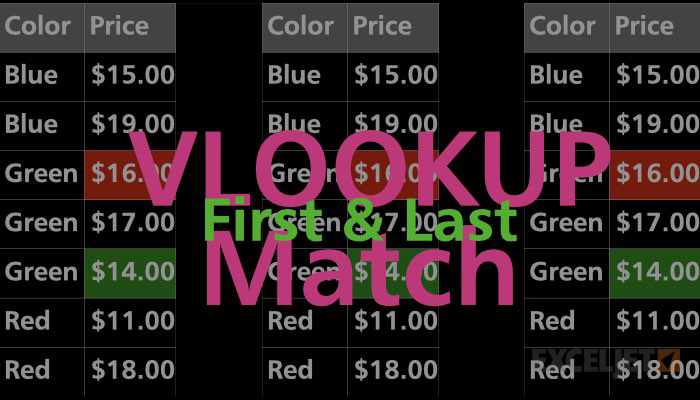
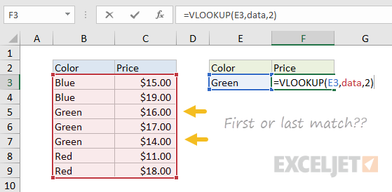
For example, if we use VLOOKUP to get the price for "green" in the data below, which price will we get?
Read on for the answer and more interesting examples.
Notes:
- The examples below use named ranges (as noted in the images) to keep formulas simple.
- Function reference links: VLOOKUP, INDEX, MATCH, and LOOKUP.
Exact match = first
When doing an exact match, you'll always get the first match, period. It doesn't matter if the data is sorted or not. In the screen below, the lookup value in E5 is "red". The VLOOKUP function, in exact match mode, returns the price for the first match:
=VLOOKUP(E5,data,2,FALSE)
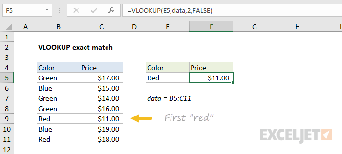
Notice the last argument in VLOOKUP is FALSE to force an exact match.
Approximate match = last
If you are doing an approximate match, and the data is sorted by lookup value, you'll get the last match. Why? Because during an approximate match, Excel scans through values until a value larger than the lookup value is found, then it "steps back" to the previous value.
In the screen below, VLOOKUP is set to approximate match mode, and colors are sorted. VLOOKUP returns the price for the last "green":
=VLOOKUP(E5,data,2,TRUE)
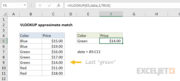
Notice the last argument in VLOOKUP is TRUE for an approximate match.
Approximate match + unsorted data = danger
With standard approximate match lookups, data must be sorted by lookup value. With unsorted data, you may see normal-looking results that are totally incorrect. This problem is more likely with VLOOKUP because VLOOKUP defaults to an approximate match when no fourth argument is provided.
To illustrate this problem, see the example below. Data is unsorted, and VLOOKUP, with no fourth argument provided, defaults to an approximate match. Notice there is no "red" with a price of $17.00, yet VLOOKUP happily returns this invalid result:
=VLOOKUP(E5,data,2)
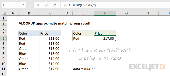
For this reason, I recommend always setting the last argument for VLOOKUP explicitly: TRUE = approximate match, FALSE = exact match. The argument is optional, but providing a value makes you think about it and provides a visual reminder in the future.
We'll look at how to overcome the problem of getting the last match and unsorted data below.
"Normal" approximate match
At this point, you may be feeling a little confused and disoriented about the idea that an approximate match can return the last match in some cases. If so, don't worry. Using an approximate match to get the last match is not the "normal" case. Typically, you'll see an approximate match used to assign values according to some kind of scale. A classic example is using VLOOKUP in approximate match mode to assign grades, which works beautifully:
=VLOOKUP(E5,key,2,TRUE)
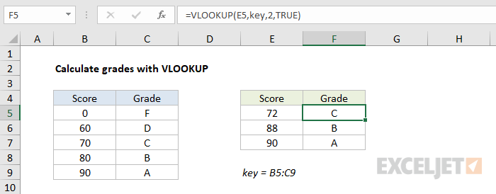
In cases like this, the lookup table deliberately does not include duplicate values, so the whole idea of "last matching value" is irrelevant. More details on this formula here.
The information above is to provide background and context for how matching works in Excel, so that the approaches described below make sense.
Practical applications
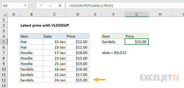
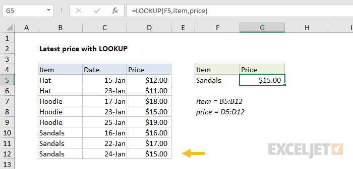
How can we use the behavior described above in a practical situation? Well, one common scenario is looking up the "latest" or "last" entry for an item. For example, below we are using VLOOKUP in approximate match mode to find the latest price for Sandals. Notice data is sorted by item, then by date, so the latest price for a given item appears last:
=VLOOKUP(F5,data,3,TRUE)
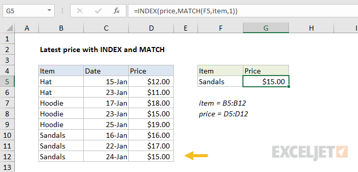
INDEX and MATCH
Other lookup functions can be used this way as well. Below, we are using an equivalent INDEX and MATCH formula to find the latest price with the same data. Notice MATCH is configured to approximate match for items sorted in ascending order by setting the third argument to 1:
=INDEX(price,MATCH(F5,item,1))
LOOKUP function
The LOOKUP function can also be used in this case. LOOKUP always performs an approximate match, so it works well in "last match" scenarios. The formula is quite simple:
=LOOKUP(F5,item,price)
Last match with unsorted data
What if you want the last match, but the data isn't sorted by lookup value? In other words, you want to apply criteria to find a match, and you simply want the last item in the data that matches your criteria? This is actually a case where the LOOKUP function shines, because LOOKUP can handle array operations natively, without control + shift + enter. This means we can dynamically build a lookup array to locate the data we want using simple logical expressions.
For example, have a look at the formula below:
=LOOKUP(2,1/(item=F5),price)
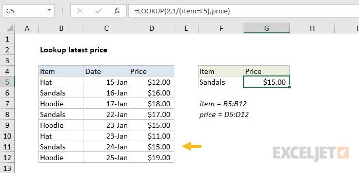
This formula finds the latest price for Sandals in unsorted data.
You may not have seen a formula like this before, so let's break it down in steps. Working from the inside out, we first apply the criteria with a simple logical expression:
item=F5
This results in an array of TRUE and FALSE values, where TRUE corresponds to items that are "sandals" and FALSE corresponds to all other values:
{FALSE;TRUE;FALSE;TRUE;FALSE;FALSE;TRUE;FALSE}
Next, we divide the number 1 by this array. During division, TRUE becomes 1, and FALSE becomes zero, so you should visualize the operation like this:
1/{0;1;0;1;0;0;1;0}
One divided by one is one, and one divided by zero is #DIV/0, so the result is another array, this one containing only 1s and #DIV/0 errors:
{#DIV/0!;1;#DIV/0!;1;#DIV/0!;#DIV/0!;1;#DIV/0!}
Don't worry, there is a method to this madness :)
Now, you may have noticed that the lookup value is the number 2. This may seem puzzling. How will LOOKUP ever find the number 2 in an array that contains only 1s and errors? It won't. We are using 2 as a lookup value to force LOOKUP to scan to the end of the data.
The LOOKUP function will automatically ignore errors, so the only thing left to match are the 1s. It will scan through the 1s looking for a 2 that will never be found. When it reaches the end of the array, it will "step back" to the last valid value – the last 1 – which corresponds to the last match based on the criteria provided.
INDEX and MATCH array version
The beauty of the LOOKUP function is that it can handle the array operation described above natively in older versions of Excel without requiring you to enter it as an array formula with Ctrl + Shift + Enter. However, you can certainly use an array formula if you like. Here is the equivalent INDEX and MATCH formula, which must be entered with control + shift + enter in older versions of Excel:
=INDEX(price,MATCH(2,1/(item=F5),1))
In a current version of Excel, the above formula will just work without special handling. Also, the newer XMATCH function and XLOOKUP function can be directly configured to return the last match.
Last non-blank cell
The approach above turns out to be really useful. For example, by tweaking the logic a bit, we can do things like find the last non-empty cell in a column:
=LOOKUP(2,1/(B:B<>""),B:B)
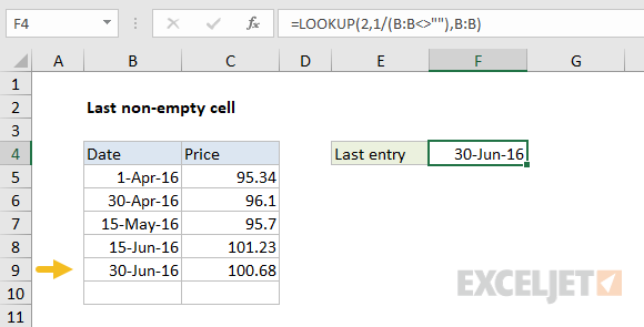
This formula is described in more detail here.
Lookup nth match? All matches?
If you've made it this far, you may be wondering how you would find the second or third match, or how you would retrieve all matches. In a modern version of Excel, the best solution is to use the FILTER function (see this page for many examples). In an older version of Excel, the formulas get significantly more complicated. Here are some examples:
- How to get nth match with VLOOKUP
- How to get nth match with INDEX and MATCH
- How to get all matches INDEX and MATCH
What's next?
Below are guides to learn more about Excel formulas. We also offer online video training.
- Formula basics - if you're just getting started
- 1000 formula examples with full explanations
- 101 important Excel functions
- 400 Excel functions
- Formula criteria - 50 examples


