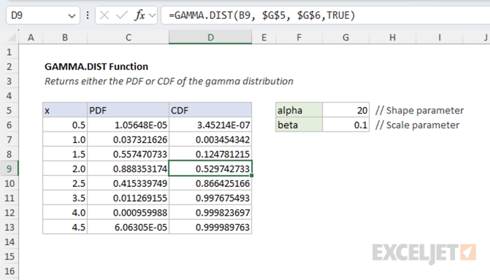
=GAMMA.DIST(x, alpha, beta, cumulative)- x - The value at which to evaluate the distribution.
- alpha - The shape parameter of the distribution.
- beta - The scale parameter of the distribution.
- cumulative - A logical value that determines the form of the function. If TRUE, returns the cumulative distribution function; if FALSE, returns the probability density function.
Using the GAMMA.DIST function
The GAMMA.DIST function calculates values for the gamma distribution, which is a continuous probability distribution commonly used in statistical analysis. The gamma distribution is particularly useful for modeling positive continuous variables and has applications in reliability analysis, queuing theory, and meteorology.
Key features
- Returns either the probability density function (PDF) or the cumulative distribution function (CDF)
- Requires all parameters to be positive numbers
- Shape parameter (alpha) controls the distribution's shape
- Scale parameter (beta) controls the distribution's spread
- Reduces to the exponential distribution when alpha = 1
- Uses a scale parameter (beta), not a rate parameter
The GAMMA.DIST function is the updated version of GAMMADIST. While GAMMADIST is still available for backward compatibility, Microsoft recommends using GAMMA.DIST for new work as it provides better accuracy.
Table of contents
- Example #1 - Farmers market stall customers
- Example #2 - Shape and scale parameters
- Example #3 - Basic probability density calculations
- Example #4 - Cumulative distribution calculations
- Example #5 - Parameter estimation
- Formula definition
- Related functions
- Notes
Example #1 - Farmers market stall customers
Suppose you work at a stall at the farmers' market. Customers appear one at a time, at random, but historical data tell you they arrive on average 10 per hour. How long will you wait until the 20th customer shows up? This scenario is a good example of when to use the gamma distribution, because it models the time until the k-th event occurs in a Poisson process (random arrivals at a constant average rate).
To set up the problem as a gamma distribution:
- Rate (λ): 10 customers per hour
- Shape parameter (alpha): 20 (the number of customers we're waiting for)
- Scale parameter (beta): 1/λ = 0.1 hours per customer
- Function type: Use CDF (cumulative = TRUE) to calculate probabilities of waiting times, rather than PDF, which gives relative likelihood at specific points
To calculate the chance of waiting ≤ x hours for the 20th customer, we calculate the probability like this:
=GAMMA.DIST(x, 20, 0.1, TRUE)
To calculate the chance of waiting > x hours for the 20th customer:
=1-GAMMA.DIST(x, 20, 0.1, TRUE)
For example, to find the probability that the 20th customer arrives in 2 hours or less, use:
=GAMMA.DIST(2, 20, 0.1, TRUE) // 53% chance of waiting ≤ 2 hours
The spreadsheet below shows different waiting times and their corresponding probabilities:
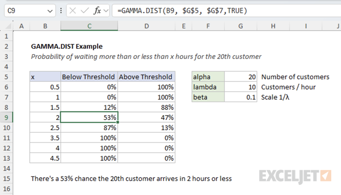
The gamma distribution is right-skewed, meaning it has a long tail to the right. This reflects the fact that while it's unlikely to wait a very long time for the 20th customer, it's still possible, due to random gaps between customer arrivals. In practice, there's a small chance you might wait far longer than average. There's also a decent chance that you'll reach 20 customers sooner than the average, which is why the probability of reaching the 20th customer at or before 2 hours is 53%, not 50%.
This skewness is more pronounced when the shape parameter α (alpha) is small. As α increases, the gamma distribution becomes more symmetric and resembles a normal distribution. The right skew is a defining characteristic of the gamma distribution that makes it well-suited for modeling real-world waiting-time problems like the one described.
Example #2 - Shape and scale parameters
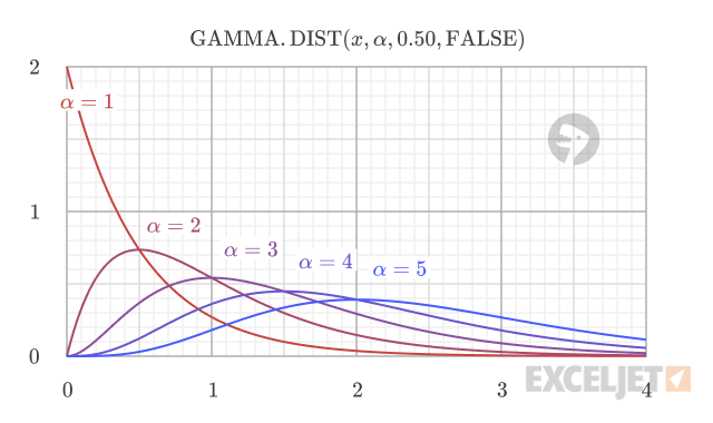
The shape parameter (alpha) controls the shape of the distribution. For lower values of alpha, the distribution is more exponential-like, with a longer tail to the right. As the value of alpha increases, the distribution becomes more symmetric and resembles a normal distribution.
The scale parameter (beta) controls the scale of the distribution. As the value of beta increases, the distribution becomes more spread out.
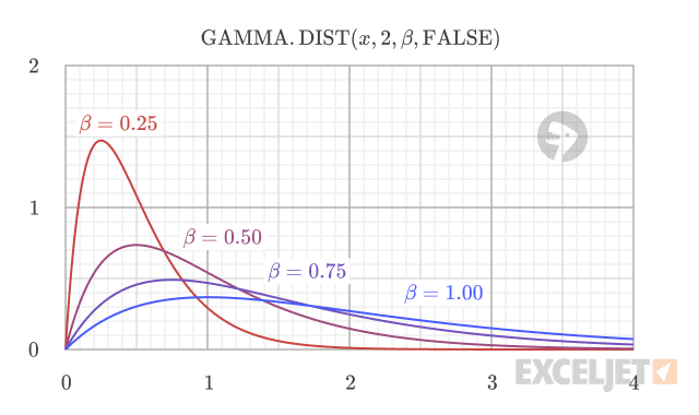
The function uses the standard parameterization where beta is the scale parameter (not rate parameter). Sometimes you'll see the gamma distribution defined with a rate parameter instead. To convert from rate to scale, use scale = 1/rate.
Example #3 - Basic probability density calculations
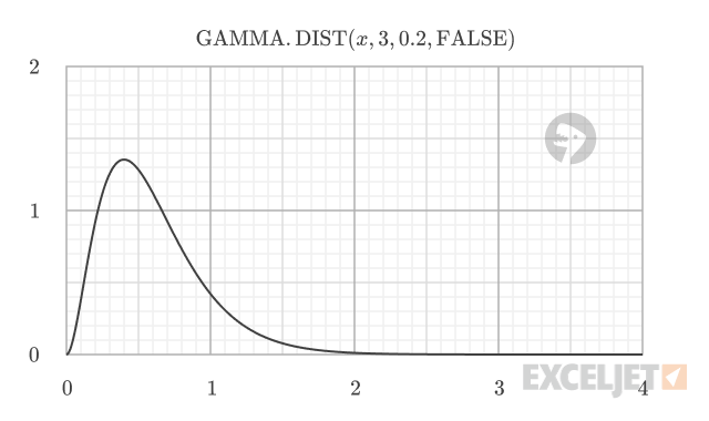
This example shows how to use GAMMA.DIST with the cumulative argument set to FALSE to calculate the probability density function (PDF). The PDF indicates the relative likelihood of a random variable taking on a value near a specific point.
In this example, we'll calculate the PDF for a gamma distribution with a shape (alpha) of 3 and a scale (beta) of 0.2. The formula is:
=GAMMA.DIST(x, 3, 0.2, FALSE)
The peak of the distribution (the mode) can be found with (alpha - 1) * beta, which is (3 - 1) * 0.2 = 0.4. We can calculate the PDF at this peak, and at other values, to see how the likelihood changes.
=GAMMA.DIST(0.4, 3, 0.2, FALSE) // returns 1.353, the peak likelihood
=GAMMA.DIST(0.2, 3, 0.2, FALSE) // returns 0.981
=GAMMA.DIST(0.8, 3, 0.2, FALSE) // returns 0.903
It's important to understand that PDF values are not probabilities. A PDF value is a measure of probability density; it indicates the relative likelihood that a random variable will be found near a particular value. A higher PDF value means it is more likely that the variable's value will be close to that point. Shown below is a graph of the PDF for the gamma distribution with alpha = 3 and beta = 0.2.
To find the actual probability of the variable falling within a specific range, you must calculate the area under the PDF curve over that interval. The area under the curve between two points represents the probability of the variable falling within that range.
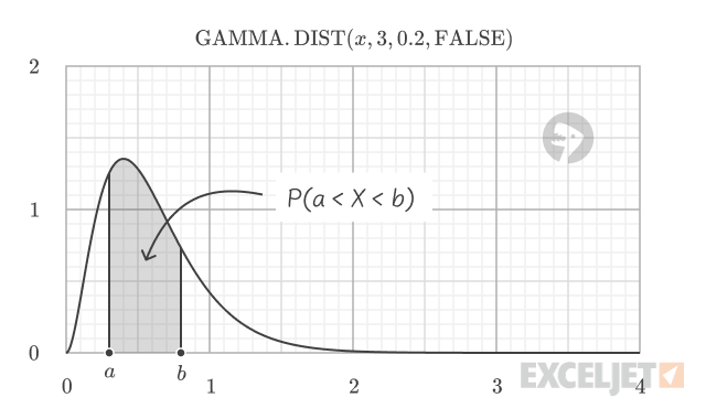
The Cumulative Distribution Function (CDF), as shown in the next example, is a practical way to compute this area.
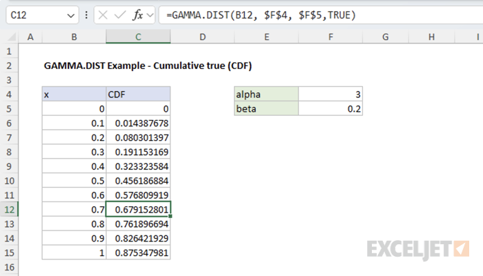
Example #4 - Cumulative distribution calculations
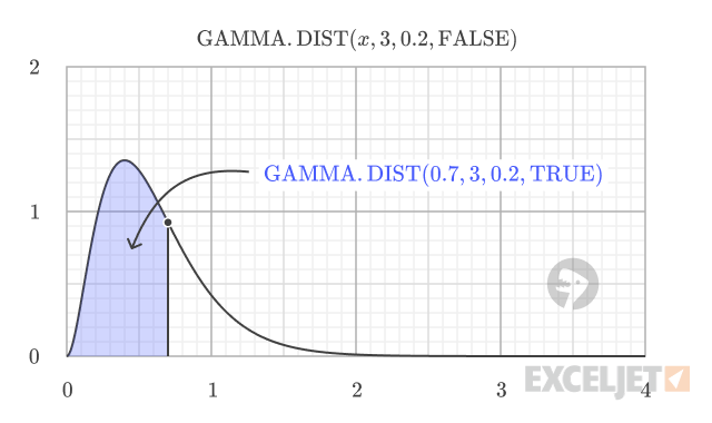
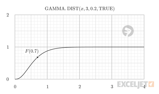
Setting the cumulative argument to TRUE returns the cumulative distribution function (CDF), which gives the probability of a random variable being less than or equal to a certain value. For example, using the same gamma distribution with alpha = 3 and beta = 0.2, the CDF at 0.7 is 0.679.
=GAMMA.DIST(0.7, 3, 0.2, TRUE) // returns 0.679
This value is equal to the area under the PDF curve to the left of 0.7.
The cumulative distribution has a characteristic S-shape. It starts at 0 for x = 0 and smoothly increases toward 1 as x grows larger, which illustrates how the probability accumulates.
To find the probability of a value falling within a specific range, we can subtract the CDF value at the lower bound from the CDF value at the upper bound.
For instance, to find the probability that a value from a gamma distribution with alpha = 3 and beta = 0.2 falls between 0.3 and 0.7, we calculate the CDF at both points and find the difference:
=GAMMA.DIST(0.7, 3, 0.2, TRUE) // P(X <= 0.7) = 0.679
=GAMMA.DIST(0.3, 3, 0.2, TRUE) // P(X <= 0.3) = 0.191
The probability of the value being between 0.3 and 0.7 is:
=GAMMA.DIST(0.7, 3, 0.2, TRUE) - GAMMA.DIST(0.3, 3, 0.2, TRUE) // returns 0.488
The spreadsheet below shows the CDF values for different values of x.
Example #5 - Parameter estimation
Sometimes you need to work backwards from sample data to estimate the gamma distribution parameters. While GAMMA.DIST doesn't directly estimate parameters, you can estimate the parameters using the method of moments.
The method of moments estimators are:
- Shape (α) = (sample mean)² / (sample variance)
- Scale (β) = (sample variance) / (sample mean)
Formula definition
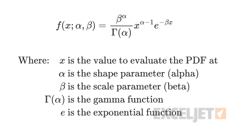
The gamma distribution is a continuous probability distribution that is defined by two parameters: the shape parameter (alpha) and the scale parameter (beta). The formula for the gamma distribution (PDF) is:
The cumulative distribution function (CDF) is the integral of the PDF from 0 to x:
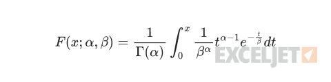
In practice, Excel calculates the GAMMA.DIST function using numerical methods. The CDF formula, in particular, involves an integral that does not have a simple, closed-form solution, so Excel uses a numerical approximation to calculate the value of the CDF.
Related functions
Excel offers several functions for working with the gamma distribution and other related probability distributions:
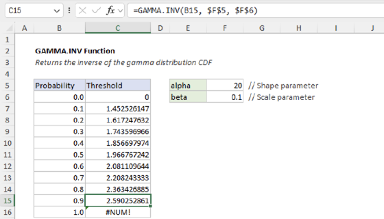
- GAMMA.INV - Calculate inverse gamma distribution (quantiles)
- GAMMALN.PRECISE - Calculate natural logarithm of gamma function
- WEIBULL.DIST - Calculate Weibull distribution (related to gamma)
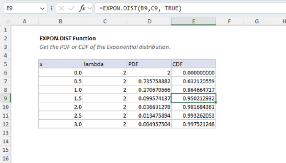
- EXPON.DIST - Calculate exponential distribution (special case of gamma)
- CHISQ.DIST - Calculate chi-squared distribution (special case of gamma)
Notes
- All parameters (x, alpha, beta) must be positive numbers
- If x < 0, the function returns #NUM! error
- If alpha ≤ 0 or beta ≤ 0, the function returns #NUM! error
- The cumulative argument must be TRUE or FALSE (or equivalent logical values)
- When alpha = 1, the gamma distribution becomes the exponential distribution
- GAMMA.DIST provides improved accuracy over the legacy GAMMADIST function
- When modeling failure rates that change over time, see WEIBULL.DIST which is often preferred for this scenario in reliability analysis.
- The chi-squared distribution is a special case of the gamma distribution where alpha = degrees of freedom / 2 and beta = 2