Sequence of times

Summary

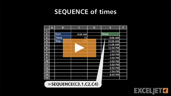
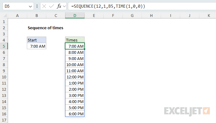
To generate a sequence of times, you can use the SEQUENCE function with the TIME function. In the example shown, the formula in D5 is:

=SEQUENCE(12,1,B5,TIME(1,0,0))

The result is 12 times, one hour apart, starting with the time in cell B5 (7:00 AM). To use a different interval, change the time given to TIME. For example, TIME(0,30,0) returns times 30 minutes apart.

Generic formula

=SEQUENCE(n,1,start,interval)

Explanation

In this example, the goal is to generate a list of times that begins at a given start time and increases by a fixed interval. The start time is in cell B5, and the result should be 12 times, one hour apart. This is a good fit for the SEQUENCE function, because in Excel, times are just numbers.

How Excel stores times
SEQUENCE function
Formatting the result
Other intervals
Exact times for lookups
Legacy Excel

How Excel stores times

In Excel, times are fractional values of a day. One whole day is 1, so 12:00 PM is 0.5, 6:00 AM is 0.25, and 7:00 AM is 7/24, or about 0.2917. One hour is 1/24 of a day, and one minute is 1/1440 of a day. This means a sequence of times is just a sequence of numbers that increase by a fixed amount, which is exactly what SEQUENCE is designed to create.

SEQUENCE function

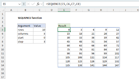
The SEQUENCE function generates a list of sequential numbers. It takes four arguments: rows, columns, start, and step. In the example shown, SEQUENCE is configured like this:

=SEQUENCE(12,1,B5,TIME(1,0,0))

rows is 12, because we want 12 times.
columns is 1, so the times are returned in a single column.
start is B5, which contains 7:00 AM.
step is TIME(1,0,0), the value for one hour.

The TIME function builds a time from separate hour, minute, and second values, so TIME(1,0,0) is one hour, TIME(0,30,0) is 30 minutes, and TIME(0,0,15) is 15 seconds. Using TIME for step makes the interval easy to read and easy to change.

SEQUENCE starts with 7:00 AM and adds one hour to each new value, so it returns an array of 12 numbers like this (rounded to four decimal places):

{0.2917;0.3333;0.375;0.4167;0.4583;0.5;0.5417;0.5833;0.625;0.6667;0.7083;0.75}

These numbers spill into the range D5:D16. Because the cells are formatted as time, the numbers appear as 7:00 AM through 6:00 PM. To list the times across a row instead of down a column, swap the first two arguments:

=SEQUENCE(1,12,B5,TIME(1,0,0))

Formatting the result

SEQUENCE returns plain numbers, so depending on how the cells are formatted, you may see decimal values like 0.291667 instead of times. This is a formatting problem, not a formula problem. To fix it, select the results and apply a time format. The keyboard shortcut Control + Shift + @ applies a time format with hours, minutes, and AM or PM, or you can apply a custom number format like h:mm AM/PM, which is the format used in the worksheet shown.

Other intervals

To change the interval, change the time given to TIME in the step argument. In the worksheet below, the start time is 8:30 AM and the formula in D5 generates times 30 minutes apart:

=SEQUENCE(12,1,B5,TIME(0,30,0))

Sequence of times 30 minutes apart

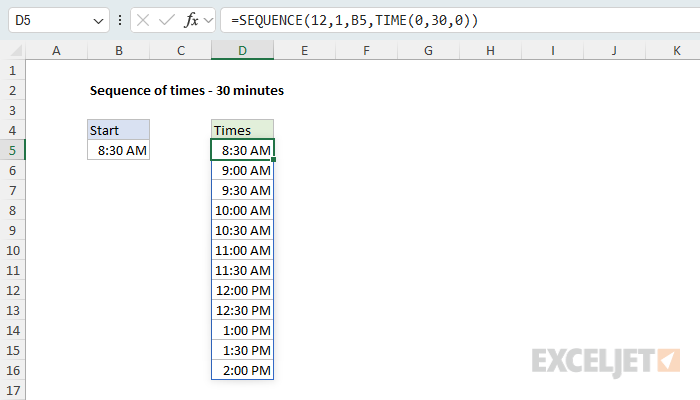
The minutes in the start time carry through, so the list begins at 8:30 AM, not 8:00 AM. Here are a few more intervals:

=SEQUENCE(12,1,B5,TIME(2,0,0)) // every 2 hours
=SEQUENCE(12,1,B5,TIME(0,15,0)) // every 15 minutes
=SEQUENCE(12,1,B5,TIME(0,5,0)) // every 5 minutes

You can also give step as a fraction of a day, since that is the number TIME returns. For example, one hour is 1/24 of a day, so this formula returns the same times as the main example:

=SEQUENCE(12,1,B5,1/24)

TIME is easier to read, especially for intervals like 15 minutes, which is 1/96 of a day.

Exact times for lookups

For most purposes, the times created by SEQUENCE are fine as they are. However, the number for one hour (1/24) can't be stored exactly in binary, so as SEQUENCE adds the step again and again, some results end up off by a tiny amount. These floating-point errors don't change how the times display, and a comparison like =D6=TIME(8,0,0) still returns TRUE, because Excel ignores tiny differences when comparing values with the equal sign.

Exact-match lookups are stricter. If you generate 12 hourly times from 7:00 AM with the formula above and look up each hour with XLOOKUP or XMATCH, 8 of the 12 lookups return #N/A. If you plan to look up the times in the list, round them to the nearest minute:

=ROUND(SEQUENCE(12,1,B5,TIME(1,0,0))*1440,0)/1440

There are 1440 minutes in a day, so multiplying by 1440 converts the times to minutes. The ROUND function removes the tiny errors, and dividing by 1440 converts the minutes back into Excel times. The results display exactly as before, but now they match times typed into a cell or created with the TIME function.

Legacy Excel

SEQUENCE is available in Excel 2021+ and Excel 365. In older versions of Excel, you can build the same list with two simple formulas. In D5, pick up the start time:

=B5

Then enter this formula in D6 and copy it down through D16:

=D5+TIME(1,0,0)

Each formula adds one hour to the time in the cell above. To use a different interval, change the time given to TIME. Adding the same step over and over creates the same tiny errors described above, so if you need exact times for lookups, round each result to the nearest minute: