Summary
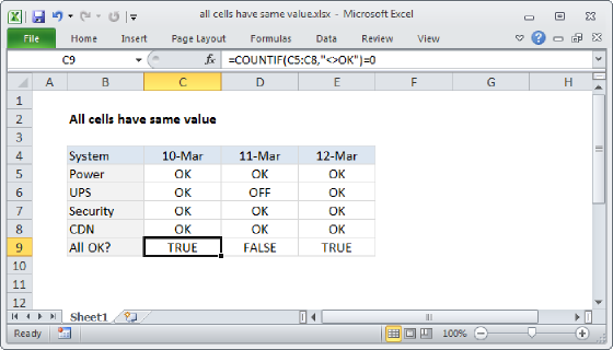
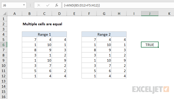
To confirm two ranges of the same size contain the same values, you can use a simple array formula based on the AND function. In the example shown, the formula in C9 is:
{=AND(B5:D12=F5:H12)}
Note: this is an array formula and must be entered with control + shift + enter.
Generic formula
{=AND(range1=range2)}
Explanation
The AND function is designed to evaluate multiple logical expressions, and returns TRUE only when all expressions are TRUE.
In this case the we simply compare one range with another with a single logical expression:
B5:D12=F5:H12
The two ranges, B5:B12 and F5:H12 are the same dimensions, 5 rows x 3 columns, each containing 15 cells. The result of this operation is an array of 15 TRUE FALSE values of the same dimensions:
{TRUE,TRUE,TRUE;
TRUE,TRUE,TRUE;
TRUE,TRUE,TRUE;
TRUE,TRUE,TRUE;
TRUE,TRUE,TRUE;
TRUE,TRUE,TRUE;
TRUE,TRUE,TRUE;
TRUE,TRUE,TRUE}
Each TRUE FALSE value is the result of comparing corresponding cells in the two arrays.
The AND function returns TRUE only if all values in the array are TRUE. In all other cases, AND will return FALSE.
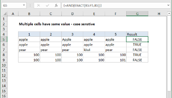
Case-sensitive option
The formula above is not case-sensitive. To compare two ranges in a case-sensitive manner, you can use a formula like this:
{=AND(EXACT(range1,range2))}
Here, the EXACT function is used to make sure the test is case-sensitive. Like the formula above, this is an array formula and must be entered with control + shift + enter.